In economics, the Gini coefficient, also known as the Gini index or Gini ratio, is a measure of statistical dispersion intended to represent the income inequality, the wealth inequality, or the consumption inequality within a nation or a social group. It was developed by Italian statistician and sociologist Corrado Gini.

Statistical inference is the process of using data analysis to infer properties of an underlying distribution of probability. Inferential statistical analysis infers properties of a population, for example by testing hypotheses and deriving estimates. It is assumed that the observed data set is sampled from a larger population.

In statistics, the standard deviation is a measure of the amount of variation or dispersion of a set of values. A low standard deviation indicates that the values tend to be close to the mean of the set, while a high standard deviation indicates that the values are spread out over a wider range.
Nonparametric statistics is a type of statistical analysis that does not rely on the assumption of a specific underlying distribution, or any other specific assumptions about the population parameters. This is in contrast to parametric statistics, which make such assumptions about the population. In nonparametric statistics, a distribution may not be specified at all, or a distribution may be specified but its parameters, such as the mean and variance, are not assumed to have a known value or distribution in advance. In some cases, parameters may be generated from the data, such as the median. Nonparametric statistics can be used for descriptive statistics or statistical inference. Nonparametric tests are often used when the assumptions of parametric tests are evidently violated.
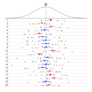
In frequentist statistics, a confidence interval (CI) is a range of estimates for an unknown parameter. A confidence interval is computed at a designated confidence level; the 95% confidence level is most common, but other levels, such as 90% or 99%, are sometimes used. The confidence level, degree of confidence or confidence coefficient represents the long-run proportion of CIs that theoretically contain the true value of the parameter; this is tantamount to the nominal coverage probability. For example, out of all intervals computed at the 95% level, 95% of them should contain the parameter's true value.
In statistics, the Mann–Whitney U test is a nonparametric test of the null hypothesis that, for randomly selected values X and Y from two populations, the probability of X being greater than Y is equal to the probability of Y being greater than X.
In statistics, an effect size is a value measuring the strength of the relationship between two variables in a population, or a sample-based estimate of that quantity. It can refer to the value of a statistic calculated from a sample of data, the value of a parameter for a hypothetical population, or to the equation that operationalizes how statistics or parameters lead to the effect size value. Examples of effect sizes include the correlation between two variables, the regression coefficient in a regression, the mean difference, or the risk of a particular event happening. Effect sizes complement statistical hypothesis testing, and play an important role in power analyses, sample size planning, and in meta-analyses. The cluster of data-analysis methods concerning effect sizes is referred to as estimation statistics.
In statistical inference, specifically predictive inference, a prediction interval is an estimate of an interval in which a future observation will fall, with a certain probability, given what has already been observed. Prediction intervals are often used in regression analysis.
The standard error (SE) of a statistic is the standard deviation of its sampling distribution or an estimate of that standard deviation. If the statistic is the sample mean, it is called the standard error of the mean (SEM). The standard error is a key ingredient in producing confidence intervals.
A tolerance interval (TI) is a statistical interval within which, with some confidence level, a specified sampled proportion of a population falls. "More specifically, a 100×p%/100×(1−α) tolerance interval provides limits within which at least a certain proportion (p) of the population falls with a given level of confidence (1−α)." "A (p, 1−α) tolerance interval (TI) based on a sample is constructed so that it would include at least a proportion p of the sampled population with confidence 1−α; such a TI is usually referred to as p-content − (1−α) coverage TI." "A (p, 1−α) upper tolerance limit (TL) is simply a 1−α upper confidence limit for the 100 p percentile of the population."
In probability theory and statistics, the coefficient of variation (CV), also known as Normalized Root-Mean-Square Deviation (NRMSD), Percent RMS, and relative standard deviation (RSD), is a standardized measure of dispersion of a probability distribution or frequency distribution. It is defined as the ratio of the standard deviation to the mean , and often expressed as a percentage ("%RSD"). The CV or RSD is widely used in analytical chemistry to express the precision and repeatability of an assay. It is also commonly used in fields such as engineering or physics when doing quality assurance studies and ANOVA gauge R&R, by economists and investors in economic models, and in psychology/neuroscience.
Sample size determination is the act of choosing the number of observations or replicates to include in a statistical sample. The sample size is an important feature of any empirical study in which the goal is to make inferences about a population from a sample. In practice, the sample size used in a study is usually determined based on the cost, time, or convenience of collecting the data, and the need for it to offer sufficient statistical power. In complicated studies there may be several different sample sizes: for example, in a stratified survey there would be different sizes for each stratum. In a census, data is sought for an entire population, hence the intended sample size is equal to the population. In experimental design, where a study may be divided into different treatment groups, there may be different sample sizes for each group.
This glossary of statistics and probability is a list of definitions of terms and concepts used in the mathematical sciences of statistics and probability, their sub-disciplines, and related fields. For additional related terms, see Glossary of mathematics and Glossary of experimental design.
A permutation test is an exact statistical hypothesis test making use of the proof by contradiction. A permutation test involves two or more samples. The null hypothesis is that all samples come from the same distribution . Under the null hypothesis, the distribution of the test statistic is obtained by calculating all possible values of the test statistic under possible rearrangements of the observed data. Permutation tests are, therefore, a form of resampling.
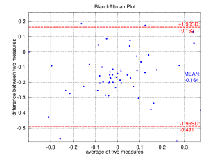
A Bland–Altman plot in analytical chemistry or biomedicine is a method of data plotting used in analyzing the agreement between two different assays. It is identical to a Tukey mean-difference plot, the name by which it is known in other fields, but was popularised in medical statistics by J. Martin Bland and Douglas G. Altman.
Bootstrapping is any test or metric that uses random sampling with replacement, and falls under the broader class of resampling methods. Bootstrapping assigns measures of accuracy to sample estimates. This technique allows estimation of the sampling distribution of almost any statistic using random sampling methods.
In probability theory and statistics, the index of dispersion, dispersion index,coefficient of dispersion,relative variance, or variance-to-mean ratio (VMR), like the coefficient of variation, is a normalized measure of the dispersion of a probability distribution: it is a measure used to quantify whether a set of observed occurrences are clustered or dispersed compared to a standard statistical model.
Exact statistics, such as that described in exact test, is a branch of statistics that was developed to provide more accurate results pertaining to statistical testing and interval estimation by eliminating procedures based on asymptotic and approximate statistical methods. The main characteristic of exact methods is that statistical tests and confidence intervals are based on exact probability statements that are valid for any sample size. Exact statistical methods help avoid some of the unreasonable assumptions of traditional statistical methods, such as the assumption of equal variances in classical ANOVA. They also allow exact inference on variance components of mixed models.
In statistics, robust measures of scale are methods that quantify the statistical dispersion in a sample of numerical data while resisting outliers. The most common such robust statistics are the interquartile range (IQR) and the median absolute deviation (MAD). These are contrasted with conventional or non-robust measures of scale, such as sample standard deviation, which are greatly influenced by outliers.
In statistics, cumulative distribution function (CDF)-based nonparametric confidence intervals are a general class of confidence intervals around statistical functionals of a distribution. To calculate these confidence intervals, all that is required is an independently and identically distributed (iid) sample from the distribution and known bounds on the support of the distribution. The latter requirement simply means that all the nonzero probability mass of the distribution must be contained in some known interval .