Self-organizing map

A self-organizing map (SOM) or self-organizing feature map (SOFM) is an unsupervised machine learning technique used to produce a low-dimensional (typically two-dimensional) representation of a higher-dimensional data set while preserving the topological structure of the data. For example, a data set with ${\displaystyle p}$ variables measured in ${\displaystyle n}$ observations could be represented as clusters of observations with similar values for the variables. These clusters then could be visualized as a two-dimensional "map" such that observations in proximal clusters have more similar values than observations in distal clusters. This can make high-dimensional data easier to visualize and analyze.

An SOM is a type of artificial neural network but is trained using competitive learning rather than the error-correction learning (e.g., backpropagation with gradient descent) used by other artificial neural networks. The SOM was introduced by the Finnish professor Teuvo Kohonen in the 1980s and therefore is sometimes called a Kohonen map or Kohonen network. ^{[1] [2]} The Kohonen map or network is a computationally convenient abstraction building on biological models of neural systems from the 1970s ^[3] and morphogenesis models dating back to Alan Turing in the 1950s. ^[4] SOMs create internal representations reminiscent of the cortical homunculus ^{[ citation needed ]}, a distorted representation of the human body, based on a neurological "map" of the areas and proportions of the human brain dedicated to processing sensory functions, for different parts of the body.

A self-organizing map showing U.S. Congress voting patterns. The input data was a table with a row for each member of Congress, and columns for certain votes containing each member's yes/no/abstain vote. The SOM algorithm arranged these members in a two-dimensional grid placing similar members closer together. The first plot shows the grouping when the data are split into two clusters. The second plot shows average distance to neighbours: larger distances are darker. The third plot predicts Republican (red) or Democratic (blue) party membership. The other plots each overlay the resulting map with predicted values on an input dimension: red means a predicted 'yes' vote on that bill, blue means a 'no' vote. The plot was created in Synapse.

Overview

Self-organizing maps, like most artificial neural networks, operate in two modes: training and mapping. First, training uses an input data set (the "input space") to generate a lower-dimensional representation of the input data (the "map space"). Second, mapping classifies additional input data using the generated map.

In most cases, the goal of training is to represent an input space with p dimensions as a map space with two dimensions. Specifically, an input space with p variables is said to have p dimensions. A map space consists of components called "nodes" or "neurons", which are arranged as a hexagonal or rectangular grid with two dimensions. ^[5] The number of nodes and their arrangement are specified beforehand based on the larger goals of the analysis and exploration of the data.

Each node in the map space is associated with a "weight" vector, which is the position of the node in the input space. While nodes in the map space stay fixed, training consists in moving weight vectors toward the input data (reducing a distance metric such as Euclidean distance) without spoiling the topology induced from the map space. After training, the map can be used to classify additional observations for the input space by finding the node with the closest weight vector (smallest distance metric) to the input space vector.

Learning algorithm

The goal of learning in the self-organizing map is to cause different parts of the network to respond similarly to certain input patterns. This is partly motivated by how visual, auditory or other sensory information is handled in separate parts of the cerebral cortex in the human brain. ^[6]

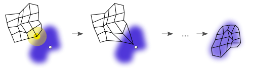
An illustration of the training of a self-organizing map. The blue blob is the distribution of the training data, and the small white disc is the current training datum drawn from that distribution. At first (left) the SOM nodes are arbitrarily positioned in the data space. The node (highlighted in yellow) which is nearest to the training datum is selected. It is moved towards the training datum, as (to a lesser extent) are its neighbors on the grid. After many iterations the grid tends to approximate the data distribution (right).

The weights of the neurons are initialized either to small random values or sampled evenly from the subspace spanned by the two largest principal component eigenvectors. With the latter alternative, learning is much faster because the initial weights already give a good approximation of SOM weights. ^[7]

The network must be fed a large number of example vectors that represent, as close as possible, the kinds of vectors expected during mapping. The examples are usually administered several times as iterations.

The training utilizes competitive learning. When a training example is fed to the network, its Euclidean distance to all weight vectors is computed. The neuron whose weight vector is most similar to the input is called the best matching unit (BMU). The weights of the BMU and neurons close to it in the SOM grid are adjusted towards the input vector. The magnitude of the change decreases with time and with the grid-distance from the BMU. The update formula for a neuron v with weight vector W_v(s) is

${\displaystyle W_{v}(s+1)=W_{v}(s)+\theta (u,v,s)\cdot \alpha (s)\cdot (D(t)-W_{v}(s))}$,

where s is the step index, t is an index into the training sample, u is the index of the BMU for the input vector D(t), α(s) is a monotonically decreasing learning coefficient; θ(u, v, s) is the neighborhood function which gives the distance between the neuron u and the neuron v in step s. ^[8] Depending on the implementations, t can scan the training data set systematically (t is 0, 1, 2...T-1, then repeat, T being the training sample's size), be randomly drawn from the data set (bootstrap sampling), or implement some other sampling method (such as jackknifing).

The neighborhood function θ(u, v, s) (also called function of lateral interaction) depends on the grid-distance between the BMU (neuron u) and neuron v. In the simplest form, it is 1 for all neurons close enough to BMU and 0 for others, but the Gaussian and Mexican-hat ^[9] functions are common choices, too. Regardless of the functional form, the neighborhood function shrinks with time. ^[6] At the beginning when the neighborhood is broad, the self-organizing takes place on the global scale. When the neighborhood has shrunk to just a couple of neurons, the weights are converging to local estimates. In some implementations, the learning coefficient α and the neighborhood function θ decrease steadily with increasing s, in others (in particular those where t scans the training data set) they decrease in step-wise fashion, once every T steps.

Training process of SOM on a two-dimensional data set

This process is repeated for each input vector for a (usually large) number of cycles λ. The network winds up associating output nodes with groups or patterns in the input data set. If these patterns can be named, the names can be attached to the associated nodes in the trained net.

During mapping, there will be one single winning neuron: the neuron whose weight vector lies closest to the input vector. This can be simply determined by calculating the Euclidean distance between input vector and weight vector.

While representing input data as vectors has been emphasized in this article, any kind of object which can be represented digitally, which has an appropriate distance measure associated with it, and in which the necessary operations for training are possible can be used to construct a self-organizing map. This includes matrices, continuous functions or even other self-organizing maps.

Algorithm

1. Randomize the node weight vectors in a map
2. For ${\displaystyle s=0,1,2,...,\lambda }$
   1. Randomly pick an input vector ${\displaystyle {D}(t)}$
   2. Find the node in the map closest to the input vector. This node is the best matching unit (BMU). Denote it by ${\displaystyle u}$
   3. For each node ${\displaystyle v}$, update its vector by pulling closer to the input vector: $${\displaystyle W_{v}(s+1)=W_{v}(s)+\theta (u,v,s)\cdot \alpha (s)\cdot (D(t)-W_{v}(s))}$$

The variable names mean the following, with vectors in bold,

• ${\displaystyle s}$ is the current iteration
• ${\displaystyle \lambda }$ is the iteration limit
• ${\displaystyle t}$ is the index of the target input data vector in the input data set ${\displaystyle \mathbf {D} }$
• ${\displaystyle {D}(t)}$ is a target input data vector
• ${\displaystyle v}$ is the index of the node in the map
• ${\displaystyle \mathbf {W} _{v}}$ is the current weight vector of node ${\displaystyle v}$
• ${\displaystyle u}$ is the index of the best matching unit (BMU) in the map
• ${\displaystyle \theta (u,v,s)}$ is the neighbourhood function,
• ${\displaystyle \alpha (s)}$ is the learning rate schedule.

The key design choices are the shape of the SOM, the neighbourhood function, and the learning rate schedule. The idea of the neighborhood function is to make it such that the BMU is updated the most, its immediate neighbors are updated a little less, and so on. The idea of the learning rate schedule is to make it so that the map updates are large at the start, and gradually stop updating.

For example, if we want to learn a SOM using a square grid, we can index it using ${\displaystyle (i,j)}$ where both ${\displaystyle i,j\in 1:N}$. The neighborhood function can make it so that the BMU updates in full, the nearest neighbors update in half, and their neighbors update in half again, etc.$${\displaystyle \theta ((i,j),(i',j'),s)={\frac {1}{2^{|i-i'|+|j-j'|}}}={\begin{cases}1&{\text{if }}i=i',j=j'\\1/2&{\text{if }}|i-i'|+|j-j'|=1\\1/4&{\text{if }}|i-i'|+|j-j'|=2\\\cdots &\cdots \end{cases}}}$$And we can use a simple linear learning rate schedule ${\displaystyle \alpha (s)=1-s/\lambda }$.

Notice in particular, that the update rate does not depend on where the point is in the Euclidean space, only on where it is in the SOM itself. For example, the points ${\displaystyle (1,1),(1,2)}$ are close on the SOM, so they will always update in similar ways, even when they are far apart on the Euclidean space. In contrast, even if the points ${\displaystyle (1,1),(1,100)}$ end up overlapping each other (such as if the SOM looks like a folded towel), they still do not update in similar ways.

Alternative algorithm

1. Randomize the map's nodes' weight vectors
2. Traverse each input vector in the input data set
   1. Traverse each node in the map
      1. Use the Euclidean distance formula to find the similarity between the input vector and the map's node's weight vector
      2. Track the node that produces the smallest distance (this node is the best matching unit, BMU)
   2. Update the nodes in the neighborhood of the BMU (including the BMU itself) by pulling them closer to the input vector
      1. ${\displaystyle W_{v}(s+1)=W_{v}(s)+\theta (u,v,s)\cdot \alpha (s)\cdot (D(t)-W_{v}(s))}$
3. Increase ${\displaystyle s}$ and repeat from step 2 while ${\displaystyle s<\lambda }$

Initialization options

Selection of initial weights as good approximations of the final weights is a well-known problem for all iterative methods of artificial neural networks, including self-organizing maps. Kohonen originally proposed random initiation of weights. ^[10] (This approach is reflected by the algorithms described above.) More recently, principal component initialization, in which initial map weights are chosen from the space of the first principal components, has become popular due to the exact reproducibility of the results. ^[11]

Cartographical representation of a self-organizing map (U-Matrix) based on Wikipedia featured article data (word frequency). Distance is inversely proportional to similarity. The "mountains" are edges between clusters. The red lines are links between articles.

A careful comparison of random initialization to principal component initialization for a one-dimensional map, however, found that the advantages of principal component initialization are not universal. The best initialization method depends on the geometry of the specific dataset. Principal component initialization was preferable (for a one-dimensional map) when the principal curve approximating the dataset could be univalently and linearly projected on the first principal component (quasilinear sets). For nonlinear datasets, however, random initiation performed better. ^[12]

Interpretation

One-dimensional SOM versus principal component analysis (PCA) for data approximation. SOM is a red broken line with squares, 20 nodes. The first principal component is presented by a blue line. Data points are the small grey circles. For PCA, the fraction of variance unexplained in this example is 23.23%, for SOM it is 6.86%.

There are two ways to interpret a SOM. Because in the training phase weights of the whole neighborhood are moved in the same direction, similar items tend to excite adjacent neurons. Therefore, SOM forms a semantic map where similar samples are mapped close together and dissimilar ones apart. This may be visualized by a U-Matrix (Euclidean distance between weight vectors of neighboring cells) of the SOM. ^{[14] [15] [16]}

The other way is to think of neuronal weights as pointers to the input space. They form a discrete approximation of the distribution of training samples. More neurons point to regions with high training sample concentration and fewer where the samples are scarce.

SOM may be considered a nonlinear generalization of Principal components analysis (PCA). ^[17] It has been shown, using both artificial and real geophysical data, that SOM has many advantages ^{[18] [19]} over the conventional feature extraction methods such as Empirical Orthogonal Functions (EOF) or PCA.

Originally, SOM was not formulated as a solution to an optimisation problem. Nevertheless, there have been several attempts to modify the definition of SOM and to formulate an optimisation problem which gives similar results. ^[20] For example, Elastic maps use the mechanical metaphor of elasticity to approximate principal manifolds: ^[21] the analogy is an elastic membrane and plate.

Examples

• Project prioritization and selection ^[22]
• Seismic facies analysis for oil and gas exploration ^[23]
• Failure mode and effects analysis ^[24]
• Finding representative data in large datasets
  • representative species for ecological communities ^[25]
  • representative days for energy system models ^[26]

Alternative approaches

• The generative topographic map (GTM) is a potential alternative to SOMs. In the sense that a GTM explicitly requires a smooth and continuous mapping from the input space to the map space, it is topology preserving. However, in a practical sense, this measure of topological preservation is lacking. ^[27]
• The growing self-organizing map (GSOM) is a growing variant of the self-organizing map. The GSOM was developed to address the issue of identifying a suitable map size in the SOM. It starts with a minimal number of nodes (usually four) and grows new nodes on the boundary based on a heuristic. By using a value called the spread factor, the data analyst has the ability to control the growth of the GSOM. ^[28]
• The conformal map approach uses conformal mapping to interpolate each training sample between grid nodes in a continuous surface. A one-to-one smooth mapping is possible in this approach. ^{[29] [30]}
• The time adaptive self-organizing map (TASOM) network is an extension of the basic SOM. The TASOM employs adaptive learning rates and neighborhood functions. It also includes a scaling parameter to make the network invariant to scaling, translation and rotation of the input space. The TASOM and its variants have been used in several applications including adaptive clustering, multilevel thresholding, input space approximation, and active contour modeling. ^[31] Moreover, a Binary Tree TASOM or BTASOM, resembling a binary natural tree having nodes composed of TASOM networks has been proposed where the number of its levels and the number of its nodes are adaptive with its environment. ^[32]
• The elastic map approach borrows from the spline interpolation the idea of minimization of the elastic energy. In learning, it minimizes the sum of quadratic bending and stretching energy with the least squares approximation error. ^[33]
• The oriented and scalable map (OS-Map) generalises the neighborhood function and the winner selection. ^[34] The homogeneous Gaussian neighborhood function is replaced with the matrix exponential. Thus one can specify the orientation either in the map space or in the data space. SOM has a fixed scale (=1), so that the maps "optimally describe the domain of observation". But what about a map covering the domain twice or in n-folds? This entails the conception of scaling. The OS-Map regards the scale as a statistical description of how many best-matching nodes an input has in the map.

See also

• Deep learning
• Hybrid Kohonen self-organizing map
• Learning vector quantization
• Liquid state machine
• Neocognitron
• Neural gas
• Sparse coding
• Sparse distributed memory
• Topological data analysis

Further reading

• Kohonen, Teuvo (January 2013). "Essentials of the self-organizing map". Neural Networks. 37: 52–65. doi:10.1016/j.neunet.2012.09.018. PMID   23067803. S2CID   17289060.
• Kohonen, Teuvo (2001). Self-organizing maps: with 22 tables. Springer Series in Information Sciences (3 ed.). Berlin Heidelberg: Springer. ISBN   978-3-540-67921-9.
• Kohonen, Teuvo (1988). "Self-Organization and Associative Memory". Springer Series in Information Sciences. 8. doi:10.1007/978-3-662-00784-6. ISBN   978-3-540-18314-3. ISSN   0720-678X.
• Kaski, Samuel, Jari Kangas, and Teuvo Kohonen. "Bibliography of self-organizing map (SOM) papers: 1981–1997." Neural computing surveys 1.3&4 (1998): 1-176.
• Oja, Merja, Samuel Kaski, and Teuvo Kohonen. "Bibliography of self-organizing map (SOM) papers: 1998–2001 addendum." Neural computing surveys 3.1 (2003): 1-156.

References

1. Kohonen, Teuvo; Honkela, Timo (2007). "Kohonen Network". Scholarpedia. 2 (1): 1568. Bibcode:2007SchpJ...2.1568K. doi: 10.4249/scholarpedia.1568 .
2. Kohonen, Teuvo (1982). "Self-Organized Formation of Topologically Correct Feature Maps". Biological Cybernetics. 43 (1): 59–69. doi:10.1007/bf00337288. S2CID   206775459.
3. Von der Malsburg, C (1973). "Self-organization of orientation sensitive cells in the striate cortex". Kybernetik. 14 (2): 85–100. doi:10.1007/bf00288907. PMID   4786750. S2CID   3351573.
4. Turing, Alan (1952). "The chemical basis of morphogenesis". Phil. Trans. R. Soc. 237 (641): 37–72. Bibcode:1952RSPTB.237...37T. doi:10.1098/rstb.1952.0012.
5. Jaakko Hollmen (9 March 1996). "Self-Organizing Map (SOM)". Aalto University .
6. Haykin, Simon (1999). "9. Self-organizing maps". Neural networks - A comprehensive foundation (2nd ed.). Prentice-Hall. ISBN   978-0-13-908385-3.
7. Kohonen, Teuvo (2005). "Intro to SOM". SOM Toolbox. Retrieved 2006-06-18.
8. Kohonen, Teuvo; Honkela, Timo (2011). "Kohonen network". Scholarpedia. 2 (1): 1568. Bibcode:2007SchpJ...2.1568K. doi: 10.4249/scholarpedia.1568 .
9. Vrieze, O.J. (1995). "Kohonen Network" (PDF). Artificial Neural Networks. Lecture Notes in Computer Science. Vol. 931. University of Limburg, Maastricht. pp. 83–100. doi:10.1007/BFb0027024. ISBN   978-3-540-59488-8 . Retrieved 1 July 2020.{{cite book}}: |website= ignored (help)
10. Kohonen, T. (2012) [1988]. Self-Organization and Associative Memory (2nd ed.). Springer. ISBN   978-3-662-00784-6.
11. Ciampi, A.; Lechevallier, Y. (2000). "Clustering large, multi-level data sets: An approach based on Kohonen self organizing maps". In Zighed, D.A.; Komorowski, J.; Zytkow, J. (eds.). Principles of Data Mining and Knowledge Discovery: 4th European Conference, PKDD 2000 Lyon, France, September 13–16, 2000 Proceedings. Lecture notes in computer science. Vol. 1910. Springer. pp. 353–358. doi: 10.1007/3-540-45372-5_36 . ISBN   3-540-45372-5.
12. Akinduko, A.A.; Mirkes, E.M.; Gorban, A.N. (2016). "SOM: Stochastic initialization versus principal components". Information Sciences. 364–365: 213–221. doi:10.1016/j.ins.2015.10.013.
13. Illustration is prepared using free software: Mirkes, Evgeny M.; Principal Component Analysis and Self-Organizing Maps: applet, University of Leicester, 2011
14. Ultsch, Alfred; Siemon, H. Peter (1990). "Kohonen's Self Organizing Feature Maps for Exploratory Data Analysis". In Widrow, Bernard; Angeniol, Bernard (eds.). Proceedings of the International Neural Network Conference (INNC-90), Paris, France, July 9–13, 1990. Vol. 1. Dordrecht, Netherlands: Kluwer. pp.  305–308. ISBN   978-0-7923-0831-7.
15. Ultsch, Alfred (2003). U*-Matrix: A tool to visualize clusters in high dimensional data (Technical report). Department of Computer Science, University of Marburg. pp. 1–12. 36.
16. Saadatdoost, Robab; Sim, Alex Tze Hiang; Jafarkarimi, Hosein (2011). "Application of self organizing map for knowledge discovery based in higher education data". Research and Innovation in Information Systems (ICRIIS), 2011 International Conference on. IEEE. doi:10.1109/ICRIIS.2011.6125693. ISBN   978-1-61284-294-3.
17. Yin, Hujun. "Learning Nonlinear Principal Manifolds by Self-Organising Maps". Gorban et al. 2008 .
18. Liu, Yonggang; Weisberg, Robert H (2005). "Patterns of Ocean Current Variability on the West Florida Shelf Using the Self-Organizing Map". Journal of Geophysical Research. 110 (C6): C06003. Bibcode:2005JGRC..110.6003L. doi: 10.1029/2004JC002786 .
19. Liu, Yonggang; Weisberg, Robert H.; Mooers, Christopher N. K. (2006). "Performance Evaluation of the Self-Organizing Map for Feature Extraction". Journal of Geophysical Research. 111 (C5): C05018. Bibcode:2006JGRC..111.5018L. doi: 10.1029/2005jc003117 .
20. Heskes, Tom (1999). "Energy Functions for Self-Organizing Maps". In Oja, Erkki; Kaski, Samuel (eds.). Kohonen Maps. Elsevier. pp. 303–315. doi:10.1016/B978-044450270-4/50024-3. ISBN   978-044450270-4.
21. Gorban, Alexander N.; Kégl, Balázs; Wunsch, Donald C.; Zinovyev, Andrei, eds. (2008). Principal Manifolds for Data Visualization and Dimension Reduction. Lecture Notes in Computer Science and Engineering. Vol. 58. Springer. ISBN   978-3-540-73749-0.
22. Zheng, G.; Vaishnavi, V. (2011). "A Multidimensional Perceptual Map Approach to Project Prioritization and Selection". AIS Transactions on Human-Computer Interaction. 3 (2): 82–103. doi: 10.17705/1thci.00028 .
23. Taner, M. T.; Walls, J. D.; Smith, M.; Taylor, G.; Carr, M. B.; Dumas, D. (2001). "Reservoir characterization by calibration of self-organized map clusters". SEG Technical Program Expanded Abstracts 2001. Vol. 2001. pp. 1552–1555. doi:10.1190/1.1816406. S2CID   59155082.
24. Chang, Wui Lee; Pang, Lie Meng; Tay, Kai Meng (March 2017). "Application of Self-Organizing Map to Failure Modes and Effects Analysis Methodology" (PDF). Neurocomputing. 249: 314–320. doi:10.1016/j.neucom.2016.04.073.
25. Park, Young-Seuk; Tison, Juliette; Lek, Sovan; Giraudel, Jean-Luc; Coste, Michel; Delmas, François (2006-11-01). "Application of a self-organizing map to select representative species in multivariate analysis: A case study determining diatom distribution patterns across France". Ecological Informatics. 4th International Conference on Ecological Informatics. 1 (3): 247–257. Bibcode:2006EcInf...1..247P. doi:10.1016/j.ecoinf.2006.03.005. ISSN   1574-9541.
26. Yilmaz, Hasan Ümitcan; Fouché, Edouard; Dengiz, Thomas; Krauß, Lucas; Keles, Dogan; Fichtner, Wolf (2019-04-01). "Reducing energy time series for energy system models via self-organizing maps". It - Information Technology. 61 (2–3): 125–133. doi:10.1515/itit-2019-0025. ISSN   2196-7032. S2CID   203160544.
27. Kaski, Samuel (1997). "Data Exploration Using Self-Organizing Maps". Acta Polytechnica Scandinavica. Mathematics, Computing and Management in Engineering Series. 82. Espoo, Finland: Finnish Academy of Technology. ISBN   978-952-5148-13-8.
28. Alahakoon, D.; Halgamuge, S.K.; Sirinivasan, B. (2000). "Dynamic Self Organizing Maps With Controlled Growth for Knowledge Discovery". IEEE Transactions on Neural Networks. 11 (3): 601–614. doi:10.1109/72.846732. PMID   18249788.
29. Liou, C.-Y.; Tai, W.-P. (2000). "Conformality in the self-organization network". Artificial Intelligence. 116 (1–2): 265–286. doi:10.1016/S0004-3702(99)00093-4.
30. Liou, C.-Y.; Kuo, Y.-T. (2005). "Conformal Self-organizing Map for a Genus Zero Manifold". The Visual Computer. 21 (5): 340–353. doi:10.1007/s00371-005-0290-6. S2CID   8677589.
31. Shah-Hosseini, Hamed; Safabakhsh, Reza (April 2003). "TASOM: A New Time Adaptive Self-Organizing Map". IEEE Transactions on Systems, Man, and Cybernetics - Part B: Cybernetics. 33 (2): 271–282. doi:10.1109/tsmcb.2003.810442. PMID   18238177.
32. Shah-Hosseini, Hamed (May 2011). "Binary Tree Time Adaptive Self-Organizing Map". Neurocomputing. 74 (11): 1823–1839. doi:10.1016/j.neucom.2010.07.037.
33. Gorban, A.N.; Zinovyev, A. (2010). "Principal manifolds and graphs in practice: from molecular biology to dynamical systems]". International Journal of Neural Systems . 20 (3): 219–232. arXiv: 1001.1122 . doi:10.1142/S0129065710002383. PMID   20556849. S2CID   2170982.
34. Hua, H (2016). "Image and geometry processing with Oriented and Scalable Map". Neural Networks. 77: 1–6. doi:10.1016/j.neunet.2016.01.009. PMID   26897100.

External links

• Media related to Self-organizing maps at Wikimedia Commons