Hierarchical clustering

"SLINK" redirects here. For the online magazine, see Slink.

In data mining and statistics, hierarchical clustering (also called hierarchical cluster analysis or HCA) is a method of cluster analysis that seeks to build a hierarchy of clusters. Strategies for hierarchical clustering generally fall into two categories:

• Agglomerative: This is a "bottom-up" approach: Each observation starts in its own cluster, and pairs of clusters are merged as one moves up the hierarchy.
• Divisive: This is a "top-down" approach: All observations start in one cluster, and splits are performed recursively as one moves down the hierarchy.

In general, the merges and splits are determined in a greedy manner. The results of hierarchical clustering ^[1] are usually presented in a dendrogram.

Hierarchical clustering has the distinct advantage that any valid measure of distance can be used. In fact, the observations themselves are not required: all that is used is a matrix of distances. On the other hand, except for the special case of single-linkage distance, none of the algorithms (except exhaustive search in ${\displaystyle {\mathcal {O}}(2^{n})}$) can be guaranteed to find the optimum solution.^{[ citation needed ]}

Complexity

The standard algorithm for hierarchical agglomerative clustering (HAC) has a time complexity of ${\displaystyle {\mathcal {O}}(n^{3})}$ and requires ${\displaystyle \Omega (n^{2})}$ memory, which makes it too slow for even medium data sets. However, for some special cases, optimal efficient agglomerative methods (of complexity ${\displaystyle {\mathcal {O}}(n^{2})}$) are known: SLINK ^[2] for single-linkage and CLINK ^[3] for complete-linkage clustering. With a heap, the runtime of the general case can be reduced to ${\displaystyle {\mathcal {O}}(n^{2}\log n)}$, an improvement on the aforementioned bound of ${\displaystyle {\mathcal {O}}(n^{3})}$, at the cost of further increasing the memory requirements. In many cases, the memory overheads of this approach are too large to make it practically usable. Methods exist which use quadtrees that demonstrate ${\displaystyle {\mathcal {O}}(n^{2})}$ total running time with ${\displaystyle {\mathcal {O}}(n)}$ space. ^[4]

Divisive clustering with an exhaustive search is ${\displaystyle {\mathcal {O}}(2^{n})}$, but it is common to use faster heuristics to choose splits, such as k-means.

Cluster Linkage

In order to decide which clusters should be combined (for agglomerative), or where a cluster should be split (for divisive), a measure of dissimilarity between sets of observations is required. In most methods of hierarchical clustering, this is achieved by use of an appropriate distance d, such as the Euclidean distance, between single observations of the data set, and a linkage criterion, which specifies the dissimilarity of sets as a function of the pairwise distances of observations in the sets. The choice of metric as well as linkage can have a major impact on the result of the clustering, where the lower level metric determines which objects are most similar, whereas the linkage criterion influences the shape of the clusters. For example, complete-linkage tends to produce more spherical clusters than single-linkage.

The linkage criterion determines the distance between sets of observations as a function of the pairwise distances between observations.

Some commonly used linkage criteria between two sets of observations A and B and a distance d are: ^{[5] [6]}

Names	Formula
Maximum or complete-linkage clustering	${\displaystyle \max _{a\in A,\,b\in B}d(a,b)}$
Minimum or single-linkage clustering	${\displaystyle \min _{a\in A,\,b\in B}d(a,b)}$
Unweighted average linkage clustering (or UPGMA)	${\displaystyle {\frac {1}{|A|\cdot |B|}}\sum _{a\in A}\sum _{b\in B}d(a,b).}$
Weighted average linkage clustering (or WPGMA)	${\displaystyle d(i\cup j,k)={\frac {d(i,k)+d(j,k)}{2}}.}$
Centroid linkage clustering, or UPGMC	${\displaystyle \lVert \mu _{A}-\mu _{B}\rVert ^{2}}$ where ${\displaystyle \mu _{A}}$ and ${\displaystyle \mu _{B}}$ are the centroids of A resp. B.
Median linkage clustering, or WPGMC	${\displaystyle d(i\cup j,k)=d(m_{i\cup j},m_{k})}$ where ${\displaystyle m_{i\cup j}={\tfrac {1}{2}}\left(m_{i}+m_{j}\right)}$
Versatile linkage clustering [7]	${\displaystyle {\sqrt[{p}]{{\frac {1}{|A|\cdot |B|}}\sum _{a\in A}\sum _{b\in B}d(a,b)^{p}}},p\neq 0}$
Ward linkage, [8] Minimum Increase of Sum of Squares (MISSQ) [9]	${\displaystyle {\frac {|A|\cdot |B|}{|A\cup B|}}\lVert \mu _{A}-\mu _{B}\rVert ^{2}=\sum _{x\in A\cup B}\lVert x-\mu _{A\cup B}\rVert ^{2}-\sum _{x\in A}\lVert x-\mu _{A}\rVert ^{2}-\sum _{x\in B}\lVert x-\mu _{B}\rVert ^{2}}$
Minimum Error Sum of Squares (MNSSQ) [9]	${\displaystyle \sum _{x\in A\cup B}\lVert x-\mu _{A\cup B}\rVert ^{2}}$
Minimum Increase in Variance (MIVAR) [9]	${\displaystyle {\frac {1}{|A\cup B|}}\sum _{x\in A\cup B}\lVert x-\mu _{A\cup B}\rVert ^{2}-{\frac {1}{|A|}}\sum _{x\in A}\lVert x-\mu _{A}\rVert ^{2}-{\frac {1}{|B|}}\sum _{x\in B}\lVert x-\mu _{B}\rVert ^{2}}$${\displaystyle ={\text{Var}}(A\cup B)-{\text{Var}}(A)-{\text{Var}}(B)}$
Minimum Variance (MNVAR) [9]	${\displaystyle {\frac {1}{|A\cup B|}}\sum _{x\in A\cup B}\lVert x-\mu _{A\cup B}\rVert ^{2}={\text{Var}}(A\cup B)}$
Hausdorff linkage [10]	${\displaystyle \max _{x\in A\cup B}\min _{y\in A\cup B}d(x,y)}$
Minimum Sum Medoid linkage [11]	${\displaystyle \min _{m\in A\cup B}\sum _{y\in A\cup B}d(m,y)}$ such that m is the medoid of the resulting cluster
Minimum Sum Increase Medoid linkage [11]	${\displaystyle \min _{m\in A\cup B}\sum _{y\in A\cup B}d(m,y)-\min _{m\in A}\sum _{y\in A}d(m,y)-\min _{m\in B}\sum _{y\in B}d(m,y)}$
Medoid linkage [12] [13]	${\displaystyle d(m_{A},m_{B})}$ where ${\displaystyle m_{A}}$, ${\displaystyle m_{B}}$ are the medoids of the previous clusters
Minimum energy clustering	${\displaystyle {\frac {2}{nm}}\sum _{i,j=1}^{n,m}\|a_{i}-b_{j}\|_{2}-{\frac {1}{n^{2}}}\sum _{i,j=1}^{n}\|a_{i}-a_{j}\|_{2}-{\frac {1}{m^{2}}}\sum _{i,j=1}^{m}\|b_{i}-b_{j}\|_{2}}$

Some of these can only be recomputed recursively (WPGMA, WPGMC), for many a recursive computation with Lance-Williams-equations is more efficient, while for other (Hausdorff, Medoid) the distances have to be computed with the slower full formula. Other linkage criteria include:

• The probability that candidate clusters spawn from the same distribution function (V-linkage).
• The product of in-degree and out-degree on a k-nearest-neighbour graph (graph degree linkage). ^[14]
• The increment of some cluster descriptor (i.e., a quantity defined for measuring the quality of a cluster) after merging two clusters. ^{[15] [16] [17]}

Agglomerative clustering example

Raw data

For example, suppose this data is to be clustered, and the Euclidean distance is the distance metric.

The hierarchical clustering dendrogram would be:

Traditional representation

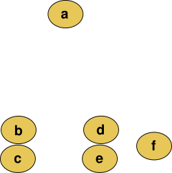
Cutting the tree at a given height will give a partitioning clustering at a selected precision. In this example, cutting after the second row (from the top) of the dendrogram will yield clusters {a} {b c} {d e} {f}. Cutting after the third row will yield clusters {a} {b c} {d e f}, which is a coarser clustering, with a smaller number but larger clusters.

This method builds the hierarchy from the individual elements by progressively merging clusters. In our example, we have six elements {a} {b} {c} {d} {e} and {f}. The first step is to determine which elements to merge in a cluster. Usually, we want to take the two closest elements, according to the chosen distance.

Optionally, one can also construct a distance matrix at this stage, where the number in the i-th row j-th column is the distance between the i-th and j-th elements. Then, as clustering progresses, rows and columns are merged as the clusters are merged and the distances updated. This is a common way to implement this type of clustering, and has the benefit of caching distances between clusters. A simple agglomerative clustering algorithm is described in the single-linkage clustering page; it can easily be adapted to different types of linkage (see below).

Suppose we have merged the two closest elements b and c, we now have the following clusters {a}, {b, c}, {d}, {e} and {f}, and want to merge them further. To do that, we need to take the distance between {a} and {b c}, and therefore define the distance between two clusters. Usually the distance between two clusters ${\displaystyle {\mathcal {A}}}$ and ${\displaystyle {\mathcal {B}}}$ is one of the following:

• The maximum distance between elements of each cluster (also called complete-linkage clustering):

${\displaystyle \max\{\,d(x,y):x\in {\mathcal {A}},\,y\in {\mathcal {B}}\,\}.}$

• The minimum distance between elements of each cluster (also called single-linkage clustering):

${\displaystyle \min\{\,d(x,y):x\in {\mathcal {A}},\,y\in {\mathcal {B}}\,\}.}$

• The mean distance between elements of each cluster (also called average linkage clustering, used e.g. in UPGMA):

${\displaystyle {1 \over {|{\mathcal {A}}|\cdot |{\mathcal {B}}|}}\sum _{x\in {\mathcal {A}}}\sum _{y\in {\mathcal {B}}}d(x,y).}$

• The sum of all intra-cluster variance.
• The increase in variance for the cluster being merged (Ward's method ^[8] )
• The probability that candidate clusters spawn from the same distribution function (V-linkage).

In case of tied minimum distances, a pair is randomly chosen, thus being able to generate several structurally different dendrograms. Alternatively, all tied pairs may be joined at the same time, generating a unique dendrogram. ^[18]

One can always decide to stop clustering when there is a sufficiently small number of clusters (number criterion). Some linkages may also guarantee that agglomeration occurs at a greater distance between clusters than the previous agglomeration, and then one can stop clustering when the clusters are too far apart to be merged (distance criterion). However, this is not the case of, e.g., the centroid linkage where the so-called reversals ^[19] (inversions, departures from ultrametricity) may occur.

Divisive clustering

The basic principle of divisive clustering was published as the DIANA (DIvisive ANAlysis clustering) algorithm. ^[20] Initially, all data is in the same cluster, and the largest cluster is split until every object is separate. Because there exist ${\displaystyle O(2^{n})}$ ways of splitting each cluster, heuristics are needed. DIANA chooses the object with the maximum average dissimilarity and then moves all objects to this cluster that are more similar to the new cluster than to the remainder.

Informally, DIANA is not so much a process of "dividing" as it is of "hollowing out": each iteration, an existing cluster (e.g. the initial cluster of the entire dataset) is chosen to form a new cluster inside of it. Objects progressively move to this nested cluster, and hollow out the existing cluster. Eventually, all that's left inside a cluster is nested clusters that grew there, without it owning any loose objects by itself.

Formally, DIANA operates in the following steps:

1. Let ${\displaystyle C_{0}=\{1\dots n\}}$ be the set of all ${\displaystyle n}$ object indices and ${\displaystyle {\mathcal {C}}=\{C_{0}\}}$ the set of all formed clusters so far.
2. Iterate the following until ${\displaystyle |{\mathcal {C}}|=n}$:
   1. Find the current cluster with 2 or more objects that has the largest diameter: ${\displaystyle C_{*}=\arg \max _{C\in {\mathcal {C}}}\max _{i_{1},i_{2}\in C}\delta (i_{1},i_{2})}$
   2. Find the object in this cluster with the most dissimilarity to the rest of the cluster: ${\displaystyle i^{*}=\arg \max _{i\in C_{*}}{\frac {1}{|C_{*}|-1}}\sum _{j\in C_{*}\setminus \{i\}}\delta (i,j)}$
   3. Pop ${\displaystyle i^{*}}$ from its old cluster ${\displaystyle C_{*}}$ and put it into a new splinter group${\displaystyle C_{\textrm {new}}=\{i^{*}\}}$.
   4. As long as ${\displaystyle C_{*}}$ isn't empty, keep migrating objects from ${\displaystyle C_{*}}$ to add them to ${\displaystyle C_{\textrm {new}}}$. To choose which objects to migrate, don't just consider dissimilarity to ${\displaystyle C_{*}}$, but also adjust for dissimilarity to the splinter group: let ${\displaystyle i^{*}=\arg \max _{i\in C}D(i)}$ where we define ${\displaystyle D(i)={\frac {1}{|C_{*}|-1}}\sum _{j\in C_{*}\setminus \{i\}}\delta (i,j)-{\frac {1}{|C_{\textrm {new}}|}}\sum _{j\in C_{\textrm {new}}}\delta (i,j)}$, then either stop iterating when ${\displaystyle D(i^{*})<0}$, or migrate ${\displaystyle i^{*}}$.
   5. Add ${\displaystyle C_{\textrm {new}}}$ to ${\displaystyle {\mathcal {C}}}$.

Intuitively, ${\displaystyle D(i)}$ above measures how strongly an object wants to leave its current cluster, but it is attenuated when the object wouldn't fit in the splinter group either. Such objects will likely start their own splinter group eventually.

The dendrogram of DIANA can be constructed by letting the splinter group ${\displaystyle C_{\textrm {new}}}$ be a child of the hollowed-out cluster ${\displaystyle C_{*}}$ each time. This constructs a tree with ${\displaystyle C_{0}}$ as its root and ${\displaystyle n}$ unique single-object clusters as its leaves.

Software

Open source implementations

Hierarchical clustering dendrogram of the Iris dataset (using R). Source

Hierarchical clustering and interactive dendrogram visualization in Orange data mining suite.

• ALGLIB implements several hierarchical clustering algorithms (single-link, complete-link, Ward) in C++ and C# with O(n²) memory and O(n³) run time.
• ELKI includes multiple hierarchical clustering algorithms, various linkage strategies and also includes the efficient SLINK, ^[2] CLINK ^[3] and Anderberg algorithms, flexible cluster extraction from dendrograms and various other cluster analysis algorithms.
• Julia has an implementation inside the Clustering.jl package. ^[21]
• Octave, the GNU analog to MATLAB implements hierarchical clustering in function "linkage".
• Orange, a data mining software suite, includes hierarchical clustering with interactive dendrogram visualisation.
• R has built-in functions ^[22] and packages that provide functions for hierarchical clustering. ^{[23] [24] [25]}
• SciPy implements hierarchical clustering in Python, including the efficient SLINK algorithm.
• scikit-learn also implements hierarchical clustering in Python.
• Weka includes hierarchical cluster analysis.

Commercial implementations

• MATLAB includes hierarchical cluster analysis.
• SAS includes hierarchical cluster analysis in PROC CLUSTER.
• Mathematica includes a Hierarchical Clustering Package.
• NCSS includes hierarchical cluster analysis.
• SPSS includes hierarchical cluster analysis.
• Qlucore Omics Explorer includes hierarchical cluster analysis.
• Stata includes hierarchical cluster analysis.
• CrimeStat includes a nearest neighbor hierarchical cluster algorithm with a graphical output for a Geographic Information System.

See also

• Binary space partitioning
• Bounding volume hierarchy
• Brown clustering
• Cladistics
• Cluster analysis
• Computational phylogenetics
• CURE data clustering algorithm
• Dasgupta's objective
• Dendrogram
• Determining the number of clusters in a data set
• Hierarchical clustering of networks
• Locality-sensitive hashing
• Nearest neighbor search
• Nearest-neighbor chain algorithm
• Numerical taxonomy
• OPTICS algorithm
• Statistical distance
• Persistent homology

References

1. Nielsen, Frank (2016). "8. Hierarchical Clustering". Introduction to HPC with MPI for Data Science. Springer. pp. 195–211. ISBN   978-3-319-21903-5.
2. R. Sibson (1973). "SLINK: an optimally efficient algorithm for the single-link cluster method" (PDF). The Computer Journal. 16 (1). British Computer Society: 30–34. doi: 10.1093/comjnl/16.1.30 .
3. D. Defays (1977). "An efficient algorithm for a complete-link method". The Computer Journal. 20 (4). British Computer Society: 364–6. doi:10.1093/comjnl/20.4.364.
4. Eppstein, David (2001-12-31). "Fast hierarchical clustering and other applications of dynamic closest pairs". ACM Journal of Experimental Algorithmics. 5: 1–es. arXiv: cs/9912014 . doi:10.1145/351827.351829. ISSN   1084-6654.
5. "The CLUSTER Procedure: Clustering Methods". SAS/STAT 9.2 Users Guide. SAS Institute . Retrieved 2009-04-26.
6. Székely, G. J.; Rizzo, M. L. (2005). "Hierarchical clustering via Joint Between-Within Distances: Extending Ward's Minimum Variance Method". Journal of Classification. 22 (2): 151–183. doi:10.1007/s00357-005-0012-9. S2CID   206960007.
7. Fernández, Alberto; Gómez, Sergio (2020). "Versatile linkage: a family of space-conserving strategies for agglomerative hierarchical clustering". Journal of Classification. 37 (3): 584–597. arXiv: 1906.09222 . doi:10.1007/s00357-019-09339-z. S2CID   195317052.
8. Ward, Joe H. (1963). "Hierarchical Grouping to Optimize an Objective Function". Journal of the American Statistical Association. 58 (301): 236–244. doi:10.2307/2282967. JSTOR   2282967. MR   0148188.
9. Podani, János (1989), Mucina, L.; Dale, M. B. (eds.), "New combinatorial clustering methods", Numerical syntaxonomy, Dordrecht: Springer Netherlands, pp. 61–77, doi:10.1007/978-94-009-2432-1_5, ISBN   978-94-009-2432-1 , retrieved 2022-11-04
10. Basalto, Nicolas; Bellotti, Roberto; De Carlo, Francesco; Facchi, Paolo; Pantaleo, Ester; Pascazio, Saverio (2007-06-15). "Hausdorff clustering of financial time series". Physica A: Statistical Mechanics and Its Applications. 379 (2): 635–644. arXiv: physics/0504014 . Bibcode:2007PhyA..379..635B. doi:10.1016/j.physa.2007.01.011. ISSN   0378-4371. S2CID   27093582.
11. Schubert, Erich (2021). HACAM: Hierarchical Agglomerative Clustering Around Medoids – and its Limitations (PDF). LWDA’21: Lernen, Wissen, Daten, Analysen September 01–03, 2021, Munich, Germany. pp. 191–204 – via CEUR-WS.
12. Miyamoto, Sadaaki; Kaizu, Yousuke; Endo, Yasunori (2016). Hierarchical and Non-Hierarchical Medoid Clustering Using Asymmetric Similarity Measures. 2016 Joint 8th International Conference on Soft Computing and Intelligent Systems (SCIS) and 17th International Symposium on Advanced Intelligent Systems (ISIS). pp. 400–403. doi:10.1109/SCIS-ISIS.2016.0091.
13. Herr, Dominik; Han, Qi; Lohmann, Steffen; Ertl, Thomas (2016). Visual Clutter Reduction through Hierarchy-based Projection of High-dimensional Labeled Data (PDF). Graphics Interface. Graphics Interface. doi:10.20380/gi2016.14 . Retrieved 2022-11-04.
14. Zhang, Wei; Wang, Xiaogang; Zhao, Deli; Tang, Xiaoou (2012). "Graph Degree Linkage: Agglomerative Clustering on a Directed Graph". In Fitzgibbon, Andrew; Lazebnik, Svetlana; Perona, Pietro; Sato, Yoichi; Schmid, Cordelia (eds.). Computer Vision – ECCV 2012. Lecture Notes in Computer Science. Vol. 7572. Springer Berlin Heidelberg. pp. 428–441. arXiv: 1208.5092 . Bibcode:2012arXiv1208.5092Z. doi:10.1007/978-3-642-33718-5_31. ISBN   9783642337185. S2CID   14751. See also: https://github.com/waynezhanghk/gacluster
15. Zhang, W.; Zhao, D.; Wang, X. (2013). "Agglomerative clustering via maximum incremental path integral". Pattern Recognition. 46 (11): 3056–65. Bibcode:2013PatRe..46.3056Z. CiteSeerX   10.1.1.719.5355 . doi:10.1016/j.patcog.2013.04.013.
16. Zhao, D.; Tang, X. (2008). "Cyclizing clusters via zeta function of a graph". NIPS'08: Proceedings of the 21st International Conference on Neural Information Processing Systems. Curran. pp. 1953–60. CiteSeerX   10.1.1.945.1649 . ISBN   9781605609492.
17. Ma, Y.; Derksen, H.; Hong, W.; Wright, J. (2007). "Segmentation of Multivariate Mixed Data via Lossy Data Coding and Compression". IEEE Transactions on Pattern Analysis and Machine Intelligence. 29 (9): 1546–62. doi:10.1109/TPAMI.2007.1085. hdl: 2142/99597 . PMID   17627043. S2CID   4591894.
18. Fernández, Alberto; Gómez, Sergio (2008). "Solving Non-uniqueness in Agglomerative Hierarchical Clustering Using Multidendrograms". Journal of Classification. 25 (1): 43–65. arXiv: cs/0608049 . doi:10.1007/s00357-008-9004-x. S2CID   434036.
19. Legendre, P.; Legendre, L.F.J. (2012). "Cluster Analysis §8.6 Reversals". Numerical Ecology. Developments in Environmental Modelling. Vol. 24 (3rd ed.). Elsevier. pp. 376–7. ISBN   978-0-444-53868-0.
20. Kaufman, L.; Rousseeuw, P.J. (2009) [1990]. "6. Divisive Analysis (Program DIANA)". Finding Groups in Data: An Introduction to Cluster Analysis. Wiley. pp. 253–279. ISBN   978-0-470-31748-8.
21. "Hierarchical Clustering · Clustering.jl". juliastats.org. Retrieved 2022-02-28.
22. "hclust function - RDocumentation". www.rdocumentation.org. Retrieved 2022-06-07.
23. Galili, Tal; Benjamini, Yoav; Simpson, Gavin; Jefferis, Gregory (2021-10-28), dendextend: Extending 'dendrogram' Functionality in R , retrieved 2022-06-07
24. Paradis, Emmanuel; et al. "ape: Analyses of Phylogenetics and Evolution" . Retrieved 2022-12-28.
25. Fernández, Alberto; Gómez, Sergio (2021-09-12). "mdendro: Extended Agglomerative Hierarchical Clustering" . Retrieved 2022-12-28.

Further reading

• Kaufman, L.; Rousseeuw, P.J. (1990). Finding Groups in Data: An Introduction to Cluster Analysis (1 ed.). New York: John Wiley. ISBN   0-471-87876-6.
• Hastie, Trevor; Tibshirani, Robert; Friedman, Jerome (2009). "14.3.12 Hierarchical clustering". The Elements of Statistical Learning (2nd ed.). New York: Springer. pp. 520–8. ISBN   978-0-387-84857-0. Archived from the original (PDF) on 2009-11-10. Retrieved 2009-10-20.