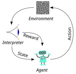
The typical framing of a reinforcement learning (RL) scenario: an agent takes actions in an environment, which is interpreted into a reward and a state representation, which are fed back to the agent.
While supervised learning and unsupervised learning algorithms respectively attempt to discover patterns in labeled and unlabeled data, reinforcement learning involves training an agent through interactions with its environment. To learn to maximize rewards from these interactions, the agent makes decisions between trying new actions to learn more about the environment (exploration), or using current knowledge of the environment to take the best action (exploitation).[1] The search for the optimal balance between these two strategies is known as the exploration–exploitation dilemma.
The environment is typically stated in the form of a Markov decision process, as many reinforcement learning algorithms use dynamic programming techniques.[2] The main difference between classical dynamic programming methods and reinforcement learning algorithms is that the latter do not assume knowledge of an exact mathematical model of the Markov decision process, and they target large Markov decision processes where exact methods become infeasible.[3]
Principles
Due to its generality, reinforcement learning is studied in many disciplines, such as game theory, control theory, operations research, information theory, simulation-based optimization, multi-agent systems, swarm intelligence, and statistics. In the operations research and control literature, RL is called approximate dynamic programming, or neuro-dynamic programming. The problems of interest in RL have also been studied in the theory of optimal control, which is concerned mostly with the existence and characterization of optimal solutions, and algorithms for their exact computation, and less with learning or approximation (particularly in the absence of a mathematical model of the environment).
A set of environment and agent states (the state space), ;
A set of actions (the action space), , of the agent;
, the transition probability (at time ) from state to state under action .
, the immediate reward after transitioning from to under action .
The purpose of reinforcement learning is for the agent to learn an optimal (or near-optimal) policy that maximizes the reward function or other user-provided reinforcement signal that accumulates from immediate rewards. This is similar to processes that appear to occur in animal psychology. For example, biological brains are hardwired to interpret signals such as pain and hunger as negative reinforcements, and interpret pleasure and food intake as positive reinforcements. In some circumstances, animals learn to adopt behaviors that optimize these rewards. This suggests that animals are capable of reinforcement learning.[4][5]
A basic reinforcement learning agent interacts with its environment in discrete time steps. At each time step t, the agent receives the current state and reward . It then chooses an action from the set of available actions, which is subsequently sent to the environment. The environment moves to a new state and the reward associated with the transition is determined. The goal of a reinforcement learning agent is to learn a policy:
that maximizes the expected cumulative reward.
Formulating the problem as a Markov decision process assumes the agent directly observes the current environmental state; in this case, the problem is said to have full observability. If the agent only has access to a subset of states, or if the observed states are corrupted by noise, the agent is said to have partial observability, and formally the problem must be formulated as a partially observable Markov decision process. In both cases, the set of actions available to the agent can be restricted. For example, the state of an account balance could be restricted to be positive; if the current value of the state is 3 and the state transition attempts to reduce the value by 4, the transition will not be allowed.
When the agent's performance is compared to that of an agent that acts optimally, the difference in performance yields the notion of regret. In order to act near optimally, the agent must reason about long-term consequences of its actions (i.e., maximize future rewards), although the immediate reward associated with this might be negative.
Two elements make reinforcement learning powerful: the use of samples to optimize performance, and the use of function approximation to deal with large environments. Thanks to these two key components, RL can be used in large environments in the following situations:
A model of the environment is known, but an analytic solution is not available;
The only way to collect information about the environment is to interact with it.
The first two of these problems could be considered planning problems (since some form of model is available), while the last one could be considered to be a genuine learning problem. However, reinforcement learning converts both planning problems to machine learning problems.
Reinforcement learning requires clever exploration mechanisms; randomly selecting actions, without reference to an estimated probability distribution, shows poor performance. The case of (small) finite Markov decision processes is relatively well understood. However, due to the lack of algorithms that scale well with the number of states (or scale to problems with infinite state spaces), simple exploration methods are the most practical.
One such method is -greedy, where is a parameter controlling the amount of exploration vs. exploitation. With probability , exploitation is chosen, and the agent chooses the action that it believes has the best long-term effect (ties between actions are broken uniformly at random). Alternatively, with probability , exploration is chosen, and the action is chosen uniformly at random. is usually a fixed parameter but can be adjusted either according to a schedule (making the agent explore progressively less), or adaptively based on heuristics.[13]
Algorithms for control learning
Even if the issue of exploration is disregarded and even if the state was observable (assumed hereafter), the problem remains to use past experience to find out which actions lead to higher cumulative rewards.
Criterion of optimality
Policy
The agent's action selection is modeled as a map called policy:
The policy map gives the probability of taking action when in state .[14]:61 There are also deterministic policies for which denotes the action that should be played at state .
State-value function
The state-value function is defined as, expected discounted return starting with state , i.e. , and successively following policy . Hence, roughly speaking, the value function estimates "how good" it is to be in a given state.[14]:60
where the random variable denotes the discounted return, and is defined as the sum of future discounted rewards:
where is the reward for transitioning from state to , is the discount rate. is less than 1, so rewards in the distant future are weighted less than rewards in the immediate future.
The algorithm must find a policy with maximum expected discounted return. From the theory of Markov decision processes it is known that, without loss of generality, the search can be restricted to the set of so-called stationary policies. A policy is stationary if the action-distribution returned by it depends only on the last state visited (from the observation agent's history). The search can be further restricted to deterministic stationary policies. A deterministic stationary policy deterministically selects actions based on the current state. Since any such policy can be identified with a mapping from the set of states to the set of actions, these policies can be identified with such mappings with no loss of generality.
For each possible policy, sample returns while following it
Choose the policy with the largest expected discounted return
One problem with this is that the number of policies can be large, or even infinite. Another is that the variance of the returns may be large, which requires many samples to accurately estimate the discounted return of each policy.
These problems can be ameliorated if we assume some structure and allow samples generated from one policy to influence the estimates made for others. The two main approaches for achieving this are value function estimation and direct policy search.
Value function approaches attempt to find a policy that maximizes the discounted return by maintaining a set of estimates of expected discounted returns for some policy (usually either the "current" [on-policy] or the optimal [off-policy] one).
These methods rely on the theory of Markov decision processes, where optimality is defined in a sense stronger than the one above: A policy is optimal if it achieves the best-expected discounted return from any initial state (i.e., initial distributions play no role in this definition). Again, an optimal policy can always be found among stationary policies.
To define optimality in a formal manner, define the state-value of a policy by
where stands for the discounted return associated with following from the initial state . Defining as the maximum possible state-value of , where is allowed to change,
A policy that achieves these optimal state-values in each state is called optimal. Clearly, a policy that is optimal in this sense is also optimal in the sense that it maximizes the expected discounted return, since , where is a state randomly sampled from the distribution of initial states (so ).
Although state-values suffice to define optimality, it is useful to define action-values. Given a state , an action and a policy , the action-value of the pair under is defined by
where now stands for the random discounted return associated with first taking action in state and following , thereafter.
The theory of Markov decision processes states that if is an optimal policy, we act optimally (take the optimal action) by choosing the action from with the highest action-value at each state, . The action-value function of such an optimal policy () is called the optimal action-value function and is commonly denoted by . In summary, the knowledge of the optimal action-value function alone suffices to know how to act optimally.
Assuming full knowledge of the Markov decision process, the two basic approaches to compute the optimal action-value function are value iteration and policy iteration. Both algorithms compute a sequence of functions () that converge to . Computing these functions involves computing expectations over the whole state-space, which is impractical for all but the smallest (finite) Markov decision processes. In reinforcement learning methods, expectations are approximated by averaging over samples and using function approximation techniques to cope with the need to represent value functions over large state-action spaces.
Monte Carlo methods
Monte Carlo methods[15] are used to solve reinforcement learning problems by averaging sample returns. Unlike methods that require full knowledge of the environment's dynamics, Monte Carlo methods rely solely on actual or simulated experience—sequences of states, actions, and rewards obtained from interaction with an environment. This makes them applicable in situations where the complete dynamics are unknown. Learning from actual experience does not require prior knowledge of the environment and can still lead to optimal behavior. When using simulated experience, only a model capable of generating sample transitions is required, rather than a full specification of transition probabilities, which is necessary for dynamic programming methods.
Monte Carlo methods apply to episodic tasks, where experience is divided into episodes that eventually terminate. Policy and value function updates occur only after the completion of an episode, making these methods incremental on an episode-by-episode basis, though not on a step-by-step (online) basis. The term "Monte Carlo" generally refers to any method involving random sampling; however, in this context, it specifically refers to methods that compute averages from complete returns, rather than partial returns.
These methods function similarly to the bandit algorithms, in which returns are averaged for each state-action pair. The key difference is that actions taken in one state affect the returns of subsequent states within the same episode, making the problem non-stationary. To address this non-stationarity, Monte Carlo methods use the framework of general policy iteration (GPI). While dynamic programming computes value functions using full knowledge of the Markov decision process, Monte Carlo methods learn these functions through sample returns. The value functions and policies interact similarly to dynamic programming to achieve optimality, first addressing the prediction problem and then extending to policy improvement and control, all based on sampled experience.[14]
The first problem is corrected by allowing the procedure to change the policy (at some or all states) before the values settle. This too may be problematic as it might prevent convergence. Most current algorithms do this, giving rise to the class of generalized policy iteration algorithms. Many actor-critic methods belong to this category.
The second issue can be corrected by allowing trajectories to contribute to any state-action pair in them. This may also help to some extent with the third problem, although a better solution when returns have high variance is Sutton's temporal difference (TD) methods that are based on the recursive Bellman equation.[16][17] The computation in TD methods can be incremental (when after each transition the memory is changed and the transition is thrown away), or batch (when the transitions are batched and the estimates are computed once based on the batch). Batch methods, such as the least-squares temporal difference method,[18] may use the information in the samples better, while incremental methods are the only choice when batch methods are infeasible due to their high computational or memory complexity. Some methods try to combine the two approaches. Methods based on temporal differences also overcome the fourth issue.
Another problem specific to TD comes from their reliance on the recursive Bellman equation. Most TD methods have a so-called parameter that can continuously interpolate between Monte Carlo methods that do not rely on the Bellman equations and the basic TD methods that rely entirely on the Bellman equations. This can be effective in palliating this issue.
Function approximation methods
In order to address the fifth issue, function approximation methods are used. Linear function approximation starts with a mapping that assigns a finite-dimensional vector to each state-action pair. Then, the action values of a state-action pair are obtained by linearly combining the components of with some weights:
The algorithms then adjust the weights, instead of adjusting the values associated with the individual state-action pairs. Methods based on ideas from nonparametric statistics (which can be seen to construct their own features) have been explored.
Value iteration can also be used as a starting point, giving rise to the Q-learning algorithm and its many variants.[19] Including Deep Q-learning methods when a neural network is used to represent Q, with various applications in stochastic search problems.[20]
The problem with using action-values is that they may need highly precise estimates of the competing action values that can be hard to obtain when the returns are noisy, though this problem is mitigated to some extent by temporal difference methods. Using the so-called compatible function approximation method compromises generality and efficiency.
Direct policy search
An alternative method is to search directly in (some subset of) the policy space, in which case the problem becomes a case of stochastic optimization. The two approaches available are gradient-based and gradient-free methods.
Gradient-based methods (policy gradient methods) start with a mapping from a finite-dimensional (parameter) space to the space of policies: given the parameter vector , let denote the policy associated to . Defining the performance function by under mild conditions this function will be differentiable as a function of the parameter vector . If the gradient of was known, one could use gradient ascent. Since an analytic expression for the gradient is not available, only a noisy estimate is available. Such an estimate can be constructed in many ways, giving rise to algorithms such as Williams's REINFORCE method[21] (which is known as the likelihood ratio method in the simulation-based optimization literature).[22]
Policy search methods may converge slowly given noisy data. For example, this happens in episodic problems when the trajectories are long and the variance of the returns is large. Value-function based methods that rely on temporal differences might help in this case. In recent years, actor–critic methods have been proposed and performed well on various problems.[23]
Policy search methods have been used in the robotics context.[24] Many policy search methods may get stuck in local optima (as they are based on local search).
Model-based algorithms
Finally, all of the above methods can be combined with algorithms that first learn a model of the Markov decision process, the probability of each next state given an action taken from an existing state. For instance, the Dyna algorithm learns a model from experience, and uses that to provide more modelled transitions for a value function, in addition to the real transitions.[25] Such methods can sometimes be extended to use of non-parametric models, such as when the transitions are simply stored and "replayed" to the learning algorithm.[26]
Model-based methods can be more computationally intensive than model-free approaches, and their utility can be limited by the extent to which the Markov decision process can be learnt.[27]
There are other ways to use models than to update a value function.[28] For instance, in model predictive control the model is used to update the behavior directly.
Theory
Both the asymptotic and finite-sample behaviors of most algorithms are well understood. Algorithms with provably good online performance (addressing the exploration issue) are known.
Efficient exploration of Markov decision processes is given in Burnetas and Katehakis (1997).[12] Finite-time performance bounds have also appeared for many algorithms, but these bounds are expected to be rather loose and thus more work is needed to better understand the relative advantages and limitations.
For incremental algorithms, asymptotic convergence issues have been settled.[clarification needed] Temporal-difference-based algorithms converge under a wider set of conditions than was previously possible (for example, when used with arbitrary, smooth function approximation).
The following table lists the key algorithms for learning a policy depending on several criteria:
The algorithm can be on-policy (it performs policy updates using trajectories sampled via the current policy)[48] or off-policy.
The action space may be discrete (e.g. the action space could be "going up", "going left", "going right", "going down", "stay") or continuous (e.g. moving the arm with a given angle).
The state space may be discrete (e.g. the agent could be in a cell in a grid) or continuous (e.g. the agent could be located at a given position in the plane).
Associative reinforcement learning tasks combine facets of stochastic learning automata tasks and supervised learning pattern classification tasks. In associative reinforcement learning tasks, the learning system interacts in a closed loop with its environment.[52]
Adversarial deep reinforcement learning is an active area of research in reinforcement learning focusing on vulnerabilities of learned policies. In this research area some studies initially showed that reinforcement learning policies are susceptible to imperceptible adversarial manipulations.[55][56][57] While some methods have been proposed to overcome these susceptibilities, in the most recent studies it has been shown that these proposed solutions are far from providing an accurate representation of current vulnerabilities of deep reinforcement learning policies.[58]
Fuzzy reinforcement learning
By introducing fuzzy inference in reinforcement learning,[59] approximating the state-action value function with fuzzy rules in continuous space becomes possible. The IF - THEN form of fuzzy rules make this approach suitable for expressing the results in a form close to natural language. Extending FRL with Fuzzy Rule Interpolation[60] allows the use of reduced size sparse fuzzy rule-bases to emphasize cardinal rules (most important state-action values).
Inverse reinforcement learning
In inverse reinforcement learning (IRL), no reward function is given. Instead, the reward function is inferred given an observed behavior from an expert. The idea is to mimic observed behavior, which is often optimal or close to optimal.[61] One popular IRL paradigm is named maximum entropy inverse reinforcement learning (MaxEnt IRL).[62] MaxEnt IRL estimates the parameters of a linear model of the reward function by maximizing the entropy of the probability distribution of observed trajectories subject to constraints related to matching expected feature counts. Recently it has been shown that MaxEnt IRL is a particular case of a more general framework named random utility inverse reinforcement learning (RU-IRL).[63] RU-IRL is based on random utility theory and Markov decision processes. While prior IRL approaches assume that the apparent random behavior of an observed agent is due to it following a random policy, RU-IRL assumes that the observed agent follows a deterministic policy but randomness in observed behavior is due to the fact that an observer only has partial access to the features the observed agent uses in decision making. The utility function is modeled as a random variable to account for the ignorance of the observer regarding the features the observed agent actually considers in its utility function.
Multi-objective reinforcement learning
Multi-objective reinforcement learning (MORL) is a form of reinforcement learning concerned with conflicting alternatives. It is distinct from multi-objective optimization in that it is concerned with agents acting in environments.[64][65]
Safe reinforcement learning
Safe reinforcement learning (SRL) can be defined as the process of learning policies that maximize the expectation of the return in problems in which it is important to ensure reasonable system performance and/or respect safety constraints during the learning and/or deployment processes.[66][67] An alternative approach is risk-averse reinforcement learning, where instead of the expected return, a risk-measure of the return is optimized, such as the conditional value at risk (CVaR).[68] In addition to mitigating risk, the CVaR objective increases robustness to model uncertainties.[69][70] However, CVaR optimization in risk-averse RL requires special care, to prevent gradient bias[71] and blindness to success.[72]
Self-reinforcement learning
Self-reinforcement learning (or self-learning), is a learning paradigm which does not use the concept of immediate reward after transition from to with action . It does not use an external reinforcement, it only uses the agent internal self-reinforcement. The internal self-reinforcement is provided by mechanism of feelings and emotions. In the learning process emotions are backpropagated by a mechanism of secondary reinforcement. The learning equation does not include the immediate reward, it only includes the state evaluation.
The self-reinforcement algorithm updates a memory matrix such that in each iteration executes the following machine learning routine:
In situation perform action .
Receive a consequence situation .
Compute state evaluation of how good is to be in the consequence situation .
Update crossbar memory .
Initial conditions of the memory are received as input from the genetic environment. It is a system with only one input (situation), and only one output (action, or behavior).
Self-reinforcement (self-learning) was introduced in 1982 along with a neural network capable of self-reinforcement learning, named Crossbar Adaptive Array (CAA).[73][74] The CAA computes, in a crossbar fashion, both decisions about actions and emotions (feelings) about consequence states. The system is driven by the interaction between cognition and emotion.[75]
Reinforcement Learning in Natural Language Processing
In recent years[when?], reinforcement learning has become a significant concept in natural language processing (NLP), where tasks are often sequential decision-making rather than static classification. Reinforcement learning is where an agent take actions in an environment to maximize the accumulation of rewards. This framework is best fit for many NLP tasks, including dialogue generation, text summarization, and machine translation, where the quality of the output depends on optimizing long-term or human-centered goals rather than the prediction of single correct label.
Early application of RL in NLP emerged in dialogue systems, where conversation was determined as a series of actions optimized for fluency and coherence. These early attempts, including policy gradient and sequence-level training techniques, laid a foundation for the broader application of reinforcement learning to other areas of NLP.
A major breakthrough happened with the introduction of reinforcement learning from human feedback (RLHF), a method in which human feedback ratings are used to train a reward model that guides the RL agent. Unlike traditional rule-based or supervised systems, RLHF allows models to align their behavior with human judgments on complex and subjective tasks. This technique was initially used in the development of InstructGPT, an effective language model trained to follow human instructions and later in ChatGPT which incorporates RLHF for improving output responses and ensuring safety.
More recently[when?], researchers have explored the use of offline RL in NLP to improve dialogue systems without the need of live human interaction. These methods optimize for user engagement, coherence, and diversity based on past conversation logs and pre-trained reward models.[76]
One example is DeepSeek-R1, which incorporates multi-stage training and cold-start data before RL. DeepSeek-R1 achieves performance comparable to OpenAI-o1-1217 on reasoning tasks. This model was trained via large-scale reinforcement learning (RL) without supervised fine-tuning (SFT) as a preliminary step. [77]
Statistical comparison of reinforcement learning algorithms
Efficient comparison of RL algorithms is essential for research, deployment and monitoring of RL systems. To compare different algorithms on a given environment, an agent can be trained for each algorithm. Since the performance is sensitive to implementation details, all algorithms should be implemented as closely as possible to each other.[78] After the training is finished, the agents can be run on a sample of test episodes, and their scores (returns) can be compared. Since episodes are typically assumed to be i.i.d, standard statistical tools can be used for hypothesis testing, such as T-test and permutation test.[79] This requires to accumulate all the rewards within an episode into a single number—the episodic return. However, this causes a loss of information, as different time-steps are averaged together, possibly with different levels of noise. Whenever the noise level varies across the episode, the statistical power can be improved significantly, by weighting the rewards according to their estimated noise.[80]
Challenges and Limitations
Despite significant advancements, reinforcement learning (RL) continues to face several challenges and limitations that hinder its widespread application in real-world scenarios.
Sample Inefficiency
RL algorithms often require a large number of interactions with the environment to learn effective policies, leading to high computational costs and time-intensive to train the agent. For instance, OpenAI's Dota-playing bot utilized thousands of years of simulated gameplay to achieve human-level performance. Techniques like experience replay and curriculum learning have been proposed to deprive sample inefficiency, but these techniques add more complexity and are not always sufficient for real-world applications.
Stability and Convergence Issues
Training RL models, particularly for deep neural network-based models, can be unstable and prone to divergence. A small change in the policy or environment can lead to extreme fluctuations in performance, making it difficult to achieve consistent results. This instability is further enhanced in the case of the continuous or high-dimensional action space, where the learning step becomes more complex and less predictable.
Generalization and Transferability
The RL agents trained in specific environments often struggle to generalize their learned policies to new, unseen scenarios. This is the major setback preventing the application of RL to dynamic real-world environments where adaptability is crucial. The challenge is to develop such algorithms that can transfer knowledge across tasks and environments without extensive retraining.
Bias and Reward Function Issues
Designing appropriate reward functions is critical in RL because poorly designed reward functions can lead to unintended behaviors. In addition, RL systems trained on biased data may perpetuate existing biases and lead to discriminatory or unfair outcomes. Both of these issues requires careful consideration of reward structures and data sources to ensure fairness and desired behaviors.
↑Russell, Stuart J.; Norvig, Peter (2010). Artificial intelligence: a modern approach (Thirded.). Upper Saddle River, New Jersey: Prentice Hall. pp.830, 831. ISBN978-0-13-604259-4.
↑Xie, Zhaoming; Hung Yu Ling; Nam Hee Kim; Michiel van de Panne (2020). "ALLSTEPS: Curriculum-driven Learning of Stepping Stone Skills". arXiv:2005.04323 [cs.GR].
↑Williams, Ronald J. (1987). "A class of gradient-estimating algorithms for reinforcement learning in neural networks". Proceedings of the IEEE First International Conference on Neural Networks. CiteSeerX10.1.1.129.8871.
↑Sutton, Richard (1990). "Integrated Architectures for Learning, Planning and Reacting based on Dynamic Programming". Machine Learning: Proceedings of the Seventh International Workshop.
↑Yamagata, Taku; McConville, Ryan; Santos-Rodriguez, Raul (2021-11-16). "Reinforcement Learning with Feedback from Multiple Humans with Diverse Skills". arXiv:2111.08596 [cs.LG].
↑Dabérius, Kevin; Granat, Elvin; Karlsson, Patrik (2020). "Deep Execution - Value and Policy Based Reinforcement Learning for Trading and Beating Market Benchmarks". The Journal of Machine Learning in Finance. 1. SSRN3374766.
↑J Duan; Y Guan; S Li (2021). "Distributional Soft Actor-Critic: Off-policy reinforcement learning for addressing value estimation errors". IEEE Transactions on Neural Networks and Learning Systems. 33 (11): 6584–6598. arXiv:2001.02811. doi:10.1109/TNNLS.2021.3082568. PMID34101599. S2CID211259373.
↑Soucek, Branko (6 May 1992). Dynamic, Genetic and Chaotic Programming: The Sixth-Generation Computer Technology Series. John Wiley & Sons, Inc. p.38. ISBN0-471-55717-X.
↑Goodfellow, Ian; Shlens, Jonathan; Szegedy, Christian (2015). "Explaining and Harnessing Adversarial Examples". International Conference on Learning Representations. arXiv:1412.6572.
↑Berenji, H.R. (1994). "Fuzzy Q-learning: A new approach for fuzzy dynamic programming". Proceedings of 1994 IEEE 3rd International Fuzzy Systems Conference. Orlando, FL, USA: IEEE. pp.486–491. doi:10.1109/FUZZY.1994.343737. ISBN0-7803-1896-X. S2CID56694947.
↑Pitombeira-Neto, Anselmo R.; Santos, Helano P.; Coelho da Silva, Ticiana L.; de Macedo, José Antonio F. (March 2024). "Trajectory modeling via random utility inverse reinforcement learning". Information Sciences. 660 120128. arXiv:2105.12092. doi:10.1016/j.ins.2024.120128. ISSN0020-0255. S2CID235187141.
↑Bozinovski, S. (1982). "A self-learning system using secondary reinforcement". In Trappl, Robert (ed.). Cybernetics and Systems Research: Proceedings of the Sixth European Meeting on Cybernetics and Systems Research. North-Holland. pp. 397–402. ISBN 978-0-444-86488-8
↑Bozinovski S. (1995) "Neuro genetic agents and structural theory of self-reinforcement learning systems". CMPSCI Technical Report 95-107, University of Massachusetts at Amherst
↑Bozinovski, S. (2014) "Modeling mechanisms of cognition-emotion interaction in artificial neural networks, since 1981." Procedia Computer Science p. 255–263
This page is based on this Wikipedia article Text is available under the CC BY-SA 4.0 license; additional terms may apply. Images, videos and audio are available under their respective licenses.