Complete-linkage clustering

For genetics, see Complete linkage

Complete-linkage clustering is one of several methods of agglomerative hierarchical clustering. At the beginning of the process, each element is in a cluster of its own. The clusters are then sequentially combined into larger clusters until all elements end up being in the same cluster. The method is also known as farthest neighbour clustering. The result of the clustering can be visualized as a dendrogram, which shows the sequence of cluster fusion and the distance at which each fusion took place. ^{[1] [2] [3]}

Clustering procedure

At each step, the two clusters separated by the shortest distance are combined. The definition of 'shortest distance' is what differentiates between the different agglomerative clustering methods. In complete-linkage clustering, the link between two clusters contains all element pairs, and the distance between clusters equals the distance between those two elements (one in each cluster) that are farthest away from each other. The shortest of these links that remains at any step causes the fusion of the two clusters whose elements are involved.

Mathematically, the complete linkage function — the distance ${\displaystyle D(X,Y)}$ between clusters ${\displaystyle X}$ and ${\displaystyle Y}$— is described by the following expression : ${\displaystyle D(X,Y)=\max _{x\in X,y\in Y}d(x,y)}$

where

• ${\displaystyle d(x,y)}$ is the distance between elements ${\displaystyle x\in X}$ and ${\displaystyle y\in Y}$ ;
• ${\displaystyle X}$ and ${\displaystyle Y}$ are two sets of elements (clusters).

Algorithms

Naive scheme

The following algorithm is an agglomerative scheme that erases rows and columns in a proximity matrix as old clusters are merged into new ones. The ${\displaystyle N\times N}$ proximity matrix D contains all distances d(i,j). The clusterings are assigned sequence numbers 0,1,......, (n − 1) and L(k) is the level of the kth clustering. A cluster with sequence number m is denoted (m) and the proximity between clusters (r) and (s) is denoted d[(r),(s)].

The complete linkage clustering algorithm consists of the following steps:

1. Begin with the disjoint clustering having level ${\displaystyle L(0)=0}$ and sequence number ${\displaystyle m=0}$.
2. Find the most similar pair of clusters in the current clustering, say pair ${\displaystyle (r),(s)}$, according to ${\displaystyle d[(r),(s)]=\max d[(i),(j)]}$where the maximum is over all pairs of clusters in the current clustering.
3. Increment the sequence number: ${\displaystyle m=m+1}$. Merge clusters ${\displaystyle (r)}$ and ${\displaystyle (s)}$ into a single cluster to form the next clustering ${\displaystyle m}$. Set the level of this clustering to ${\displaystyle L(m)=d[(r),(s)]}$
4. Update the proximity matrix, ${\displaystyle D}$, by deleting the rows and columns corresponding to clusters ${\displaystyle (r)}$ and ${\displaystyle (s)}$ and adding a row and column corresponding to the newly formed cluster. The proximity between the new cluster, denoted ${\displaystyle (r,s)}$, and an old cluster ${\displaystyle (k)}$ is defined as ${\displaystyle d[(r,s),(k)]=\max\{d[(k),(r)],d[(k),(s)]\}}$.
5. If all objects are in one cluster, stop. Else, go to step 2.

Optimally efficient scheme

The algorithm explained above is easy to understand but of complexity ${\displaystyle O(n^{3})}$. In May 1976, D. Defays proposed an optimally efficient algorithm of only complexity ${\displaystyle O(n^{2})}$ known as CLINK (published 1977) ^[4] inspired by the similar algorithm SLINK for single-linkage clustering.

Working example

The working example is based on a JC69 genetic distance matrix computed from the 5S ribosomal RNA sequence alignment of five bacteria: Bacillus subtilis (${\displaystyle a}$), Bacillus stearothermophilus (${\displaystyle b}$), Lactobacillus viridescens (${\displaystyle c}$), Acholeplasma modicum (${\displaystyle d}$), and Micrococcus luteus (${\displaystyle e}$). ^{[5] [6]}

First step

• First clustering

Let us assume that we have five elements ${\displaystyle (a,b,c,d,e)}$ and the following matrix ${\displaystyle D_{1}}$ of pairwise distances between them:

	a	b	c	d	e
a	0	17	21	31	23
b	17	0	30	34	21
c	21	30	0	28	39
d	31	34	28	0	43
e	23	21	39	43	0

In this example, ${\displaystyle D_{1}(a,b)=17}$ is the smallest value of ${\displaystyle D_{1}}$, so we join elements ${\displaystyle a}$ and ${\displaystyle b}$.

• First branch length estimation

Let ${\displaystyle u}$ denote the node to which ${\displaystyle a}$ and ${\displaystyle b}$ are now connected. Setting ${\displaystyle \delta (a,u)=\delta (b,u)=D_{1}(a,b)/2}$ ensures that elements ${\displaystyle a}$ and ${\displaystyle b}$ are equidistant from ${\displaystyle u}$. This corresponds to the expectation of the ultrametricity hypothesis. The branches joining ${\displaystyle a}$ and ${\displaystyle b}$ to ${\displaystyle u}$ then have lengths ${\displaystyle \delta (a,u)=\delta (b,u)=17/2=8.5}$ ( see the final dendrogram )

• First distance matrix update

We then proceed to update the initial proximity matrix ${\displaystyle D_{1}}$ into a new proximity matrix ${\displaystyle D_{2}}$ (see below), reduced in size by one row and one column because of the clustering of ${\displaystyle a}$ with ${\displaystyle b}$. Bold values in ${\displaystyle D_{2}}$ correspond to the new distances, calculated by retaining the maximum distance between each element of the first cluster ${\displaystyle (a,b)}$ and each of the remaining elements:

${\displaystyle D_{2}((a,b),c)=max(D_{1}(a,c),D_{1}(b,c))=max(21,30)=30}$

${\displaystyle D_{2}((a,b),d)=max(D_{1}(a,d),D_{1}(b,d))=max(31,34)=34}$

${\displaystyle D_{2}((a,b),e)=max(D_{1}(a,e),D_{1}(b,e))=max(23,21)=23}$

Italicized values in ${\displaystyle D_{2}}$ are not affected by the matrix update as they correspond to distances between elements not involved in the first cluster.

Second step

• Second clustering

We now reiterate the three previous steps, starting from the new distance matrix ${\displaystyle D_{2}}$ :

	(a,b)	c	d	e
(a,b)	0	30	34	23
c	30	0	28	39
d	34	28	0	43
e	23	39	43	0

Here, ${\displaystyle D_{2}((a,b),e)=23}$ is the lowest value of ${\displaystyle D_{2}}$, so we join cluster ${\displaystyle (a,b)}$ with element ${\displaystyle e}$.

• Second branch length estimation

Let ${\displaystyle v}$ denote the node to which ${\displaystyle (a,b)}$ and ${\displaystyle e}$ are now connected. Because of the ultrametricity constraint, the branches joining ${\displaystyle a}$ or ${\displaystyle b}$ to ${\displaystyle v}$, and ${\displaystyle e}$ to ${\displaystyle v}$, are equal and have the following total length: ${\displaystyle \delta (a,v)=\delta (b,v)=\delta (e,v)=23/2=11.5}$

We deduce the missing branch length: ${\displaystyle \delta (u,v)=\delta (e,v)-\delta (a,u)=\delta (e,v)-\delta (b,u)=11.5-8.5=3}$ ( see the final dendrogram )

• Second distance matrix update

We then proceed to update the ${\displaystyle D_{2}}$ matrix into a new distance matrix ${\displaystyle D_{3}}$ (see below), reduced in size by one row and one column because of the clustering of ${\displaystyle (a,b)}$ with ${\displaystyle e}$ :

${\displaystyle D_{3}(((a,b),e),c)=max(D_{2}((a,b),c),D_{2}(e,c))=max(30,39)=39}$

${\displaystyle D_{3}(((a,b),e),d)=max(D_{2}((a,b),d),D_{2}(e,d))=max(34,43)=43}$

Third step

• Third clustering

We again reiterate the three previous steps, starting from the updated distance matrix ${\displaystyle D_{3}}$.

	((a,b),e)	c	d
((a,b),e)	0	39	43
c	39	0	28
d	43	28	0

Here, ${\displaystyle D_{3}(c,d)=28}$ is the smallest value of ${\displaystyle D_{3}}$, so we join elements ${\displaystyle c}$ and ${\displaystyle d}$.

• Third branch length estimation

Let ${\displaystyle w}$ denote the node to which ${\displaystyle c}$ and ${\displaystyle d}$ are now connected. The branches joining ${\displaystyle c}$ and ${\displaystyle d}$ to ${\displaystyle w}$ then have lengths ${\displaystyle \delta (c,w)=\delta (d,w)=28/2=14}$ ( see the final dendrogram )

• Third distance matrix update

There is a single entry to update: ${\displaystyle D_{4}((c,d),((a,b),e))=max(D_{3}(c,((a,b),e)),D_{3}(d,((a,b),e)))=max(39,43)=43}$

Final step

The final ${\displaystyle D_{4}}$ matrix is:

	((a,b),e)	(c,d)
((a,b),e)	0	43
(c,d)	43	0

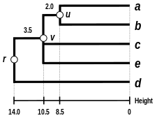
So we join clusters ${\displaystyle ((a,b),e)}$ and ${\displaystyle (c,d)}$.

Let ${\displaystyle r}$ denote the (root) node to which ${\displaystyle ((a,b),e)}$ and ${\displaystyle (c,d)}$ are now connected. The branches joining ${\displaystyle ((a,b),e)}$ and ${\displaystyle (c,d)}$ to ${\displaystyle r}$ then have lengths:

${\displaystyle \delta (((a,b),e),r)=\delta ((c,d),r)=43/2=21.5}$

We deduce the two remaining branch lengths:

${\displaystyle \delta (v,r)=\delta (((a,b),e),r)-\delta (e,v)=21.5-11.5=10}$

${\displaystyle \delta (w,r)=\delta ((c,d),r)-\delta (c,w)=21.5-14=7.5}$

The complete-linkage dendrogram

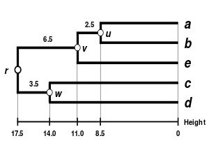
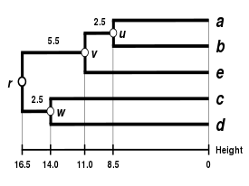
WPGMA Dendrogram 5S data

The dendrogram is now complete. It is ultrametric because all tips (${\displaystyle a}$ to ${\displaystyle e}$) are equidistant from ${\displaystyle r}$ :

${\displaystyle \delta (a,r)=\delta (b,r)=\delta (e,r)=\delta (c,r)=\delta (d,r)=21.5}$

The dendrogram is therefore rooted by ${\displaystyle r}$, its deepest node.

Comparison with other linkages

Alternative linkage schemes include single linkage clustering and average linkage clustering - implementing a different linkage in the naive algorithm is simply a matter of using a different formula to calculate inter-cluster distances in the initial computation of the proximity matrix and in step 4 of the above algorithm. An optimally efficient algorithm is however not available for arbitrary linkages. The formula that should be adjusted has been highlighted using bold text.

Complete linkage clustering avoids a drawback of the alternative single linkage method - the so-called chaining phenomenon, where clusters formed via single linkage clustering may be forced together due to single elements being close to each other, even though many of the elements in each cluster may be very distant to each other. Complete linkage tends to find compact clusters of approximately equal diameters. ^[7]

Comparison of dendrograms obtained under different clustering methods from the same distance matrix.

Single-linkage clustering.	Complete-linkage clustering.	Average linkage clustering: WPGMA.	Average linkage clustering: UPGMA.

See also

• Cluster analysis
• Hierarchical clustering
• Molecular clock
• Neighbor-joining
• Single-linkage clustering
• UPGMA
• WPGMA

References

1. Sorensen T (1948). "A method of establishing groups of equal amplitude in plant sociology based on similarity of species and its application to analyses of the vegetation on Danish commons". Biologiske Skrifter. 5: 1–34.
2. Legendre P, Legendre L (1998). Numerical Ecology (Second English ed.). p. 853.
3. Everitt BS, Landau S, Leese M (2001). Cluster Analysis (Fourth ed.). London: Arnold. ISBN   0-340-76119-9.
4. Defays D (1977). "An efficient algorithm for a complete link method". The Computer Journal. British Computer Society. 20 (4): 364–366. doi:10.1093/comjnl/20.4.364.
5. Erdmann VA, Wolters J (1986). "Collection of published 5S, 5.8S and 4.5S ribosomal RNA sequences". Nucleic Acids Research. 14 Suppl (Suppl): r1-59. doi:10.1093/nar/14.suppl.r1. PMC   341310 . PMID   2422630.
6. Olsen GJ (1988). Phylogenetic analysis using ribosomal RNA. Methods in Enzymology. Vol. 164. pp. 793–812. doi:10.1016/s0076-6879(88)64084-5. PMID   3241556.
7. Everitt, Landau and Leese (2001), pp. 62-64.

Further reading

• Späth H (1980). Cluster Analysis Algorithms. Chichester: Ellis Horwood.