
A self-organizing map (SOM) or self-organizing feature map (SOFM) is an unsupervised machine learning technique used to produce a low-dimensional representation of a higher dimensional data set while preserving the topological structure of the data. For example, a data set with variables measured in observations could be represented as clusters of observations with similar values for the variables. These clusters then could be visualized as a two-dimensional "map" such that observations in proximal clusters have more similar values than observations in distal clusters. This can make high-dimensional data easier to visualize and analyze.

In machine learning, the perceptron is an algorithm for supervised learning of binary classifiers. A binary classifier is a function which can decide whether or not an input, represented by a vector of numbers, belongs to some specific class. It is a type of linear classifier, i.e. a classification algorithm that makes its predictions based on a linear predictor function combining a set of weights with the feature vector.
Unsupervised learning, is paradigm in machine learning where, in contrast to supervised learning and semi-supervised learning, algorithms learn patterns exclusively from unlabeled data.

Nonlinear dimensionality reduction, also known as manifold learning, refers to various related techniques that aim to project high-dimensional data onto lower-dimensional latent manifolds, with the goal of either visualizing the data in the low-dimensional space, or learning the mapping itself. The techniques described below can be understood as generalizations of linear decomposition methods used for dimensionality reduction, such as singular value decomposition and principal component analysis.
In computer science, learning vector quantization (LVQ) is a prototype-based supervised classification algorithm. LVQ is the supervised counterpart of vector quantization systems.
As a machine-learning algorithm, backpropagation performs a backward pass to adjust the model's parameters, aiming to minimize the mean squared error (MSE). In a single-layered network, backpropagation uses the following steps:
- Traverse through the network from the input to the output by computing the hidden layers' output and the output layer.
- In the output layer, calculate the derivative of the cost function with respect to the input and the hidden layers.
- Repeatedly update the weights until they converge or the model has undergone enough iterations.
In abstract algebra, the split-quaternions or coquaternions form an algebraic structure introduced by James Cockle in 1849 under the latter name. They form an associative algebra of dimension four over the real numbers.
In mathematics, the Grothendieck group, or group of differences, of a commutative monoid M is a certain abelian group. This abelian group is constructed from M in the most universal way, in the sense that any abelian group containing a homomorphic image of M will also contain a homomorphic image of the Grothendieck group of M. The Grothendieck group construction takes its name from a specific case in category theory, introduced by Alexander Grothendieck in his proof of the Grothendieck–Riemann–Roch theorem, which resulted in the development of K-theory. This specific case is the monoid of isomorphism classes of objects of an abelian category, with the direct sum as its operation.
Neural gas is an artificial neural network, inspired by the self-organizing map and introduced in 1991 by Thomas Martinetz and Klaus Schulten. The neural gas is a simple algorithm for finding optimal data representations based on feature vectors. The algorithm was coined "neural gas" because of the dynamics of the feature vectors during the adaptation process, which distribute themselves like a gas within the data space. It is applied where data compression or vector quantization is an issue, for example speech recognition, image processing or pattern recognition. As a robustly converging alternative to the k-means clustering it is also used for cluster analysis.
In mathematics, a super vector space is a -graded vector space, that is, a vector space over a field with a given decomposition of subspaces of grade and grade . The study of super vector spaces and their generalizations is sometimes called super linear algebra. These objects find their principal application in theoretical physics where they are used to describe the various algebraic aspects of supersymmetry.
Oja's learning rule, or simply Oja's rule, named after Finnish computer scientist Erkki Oja, is a model of how neurons in the brain or in artificial neural networks change connection strength, or learn, over time. It is a modification of the standard Hebb's Rule that, through multiplicative normalization, solves all stability problems and generates an algorithm for principal components analysis. This is a computational form of an effect which is believed to happen in biological neurons.
In mathematics, the classical groups are defined as the special linear groups over the reals R, the complex numbers C and the quaternions H together with special automorphism groups of symmetric or skew-symmetric bilinear forms and Hermitian or skew-Hermitian sesquilinear forms defined on real, complex and quaternionic finite-dimensional vector spaces. Of these, the complex classical Lie groups are four infinite families of Lie groups that together with the exceptional groups exhaust the classification of simple Lie groups. The compact classical groups are compact real forms of the complex classical groups. The finite analogues of the classical groups are the classical groups of Lie type. The term "classical group" was coined by Hermann Weyl, it being the title of his 1939 monograph The Classical Groups.
The generalized Hebbian algorithm (GHA), also known in the literature as Sanger's rule, is a linear feedforward neural network model for unsupervised learning with applications primarily in principal components analysis. First defined in 1989, it is similar to Oja's rule in its formulation and stability, except it can be applied to networks with multiple outputs. The name originates because of the similarity between the algorithm and a hypothesis made by Donald Hebb about the way in which synaptic strengths in the brain are modified in response to experience, i.e., that changes are proportional to the correlation between the firing of pre- and post-synaptic neurons.
Competitive learning is a form of unsupervised learning in artificial neural networks, in which nodes compete for the right to respond to a subset of the input data. A variant of Hebbian learning, competitive learning works by increasing the specialization of each node in the network. It is well suited to finding clusters within data.
The U-matrix is a representation of a self-organizing map (SOM) where the Euclidean distance between the codebook vectors of neighboring neurons is depicted in a grayscale image. This image is used to visualize the data in a high-dimensional space using a 2D image.
Extension neural network is a pattern recognition method found by M. H. Wang and C. P. Hung in 2003 to classify instances of data sets. Extension neural network is composed of artificial neural network and extension theory concepts. It uses the fast and adaptive learning capability of neural network and correlation estimation property of extension theory by calculating extension distance.
ENN was used in:
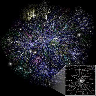
In graph theory, the Katz centrality or alpha centrality of a node is a measure of centrality in a network. It was introduced by Leo Katz in 1953 and is used to measure the relative degree of influence of an actor within a social network. Unlike typical centrality measures which consider only the shortest path between a pair of actors, Katz centrality measures influence by taking into account the total number of walks between a pair of actors.

A restricted Boltzmann machine (RBM) is a generative stochastic artificial neural network that can learn a probability distribution over its set of inputs.
Fusion adaptive resonance theory (fusion ART) is a generalization of self-organizing neural networks known as the original Adaptive Resonance Theory models for learning recognition categories (or cognitive codes) across multiple pattern channels. There is a separate stream of work on fusion ARTMAP, that extends fuzzy ARTMAP consisting of two fuzzy ART modules connected by an inter-ART map field to an extended architecture consisting of multiple ART modules.
A Transformer is a deep learning architecture that relies on the attention mechanism. It is notable for requiring less training time compared to previous recurrent neural architectures, such as long short-term memory (LSTM), and has been prevalently adopted for training large language models on large (language) datasets, such as the Wikipedia Corpus and Common Crawl, by virtue of the parallelized processing of input sequence. More specifically, the model takes in tokenized input tokens, and at each layer, contextualizes each token with other (unmasked) input tokens in parallel via attention mechanism. Though the Transformer model came out in 2017, the core attention mechanism was proposed earlier in 2014 by Bahdanau, Cho, and Bengio for machine translation. This architecture is now used not only in natural language processing, computer vision, but also in audio, and multi-modal processing. It has also led to the development of pre-trained systems, such as generative pre-trained transformers (GPTs) and BERT.


