Finite element method

"Finite element" redirects here. For the elements of a poset, see compact element.

Visualization of how a car deforms in an asymmetrical crash using finite element analysis

The finite element method (FEM) is a popular method for numerically solving differential equations arising in engineering and mathematical modeling. Typical problem areas of interest include the traditional fields of structural analysis, heat transfer, fluid flow, mass transport, and electromagnetic potential.

The FEM is a general numerical method for solving partial differential equations in two or three space variables (i.e., some boundary value problems). To solve a problem, the FEM subdivides a large system into smaller, simpler parts called finite elements. This is achieved by a particular space discretization in the space dimensions, which is implemented by the construction of a mesh of the object: the numerical domain for the solution, which has a finite number of points. The finite element method formulation of a boundary value problem finally results in a system of algebraic equations. The method approximates the unknown function over the domain. ^[1] The simple equations that model these finite elements are then assembled into a larger system of equations that models the entire problem. The FEM then approximates a solution by minimizing an associated error function via the calculus of variations.

Studying or analyzing a phenomenon with FEM is often referred to as finite element analysis (FEA).

Basic concepts

FEM mesh created by an analyst before finding a solution to a magnetic problem using FEM software. Colors indicate that the analyst has set material properties for each zone, in this case, a conducting wire coil in orange; a ferromagnetic component (perhaps iron) in light blue; and air in grey. Although the geometry may seem simple, it would be very challenging to calculate the magnetic field for this setup without FEM software using equations alone.

FEM solution to the problem at left, involving a cylindrically shaped magnetic shield. The ferromagnetic cylindrical part shields the area inside the cylinder by diverting the magnetic field created by the coil (rectangular area on the right). The color represents the amplitude of the magnetic flux density, as indicated by the scale in the inset legend, red being high amplitude. The area inside the cylinder is low amplitude (dark blue, with widely spaced lines of magnetic flux), which suggests that the shield is performing as it was designed to.

The subdivision of a whole domain into simpler parts has several advantages: ^[2]

• Accurate representation of complex geometry
• Inclusion of dissimilar material properties
• Easy representation of the total solution
• Capture of local effects.

Typical work out of the method involves:

1. dividing the domain of the problem into a collection of subdomains, with each subdomain represented by a set of element equations to the original problem
2. systematically recombining all sets of element equations into a global system of equations for the final calculation.

The global system of equations has known solution techniques and can be calculated from the initial values of the original problem to obtain a numerical answer.

In the first step above, the element equations are simple equations that locally approximate the original complex equations to be studied, where the original equations are often partial differential equations (PDE). To explain the approximation in this process, the finite element method is commonly introduced as a special case of Galerkin method. The process, in mathematical language, is to construct an integral of the inner product of the residual and the weight functions and set the integral to zero. In simple terms, it is a procedure that minimizes the approximation error by fitting trial functions into the PDE. The residual is the error caused by the trial functions, and the weight functions are polynomial approximation functions that project the residual. The process eliminates all the spatial derivatives from the PDE, thus approximating the PDE locally with

• a set of algebraic equations for steady state problems,
• a set of ordinary differential equations for transient problems.

These equation sets are element equations. They are linear if the underlying PDE is linear and vice versa. Algebraic equation sets that arise in the steady-state problems are solved using numerical linear algebra methods. In contrast, ordinary differential equation sets that occur in the transient problems are solved by numerical integration using standard techniques such as Euler's method or the Runge-Kutta method.

In step (2) above, a global system of equations is generated from the element equations by transforming coordinates from the subdomains' local nodes to the domain's global nodes. This spatial transformation includes appropriate orientation adjustments as applied in relation to the reference coordinate system. The process is often carried out by FEM software using coordinate data generated from the subdomains.

The practical application of FEM is known as finite element analysis (FEA). FEA as applied in engineering, is a computational tool for performing engineering analysis. It includes the use of mesh generation techniques for dividing a complex problem into small elements, as well as the use of software coded with a FEM algorithm. In applying FEA, the complex problem is usually a physical system with the underlying physics such as the Euler–Bernoulli beam equation, the heat equation, or the Navier-Stokes equations expressed in either PDE or integral equations, while the divided small elements of the complex problem represent different areas in the physical system.

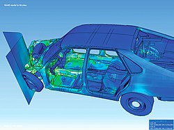
FEA may be used for analyzing problems over complicated domains (like cars and oil pipelines) when the domain changes (as during a solid-state reaction with a moving boundary), when the desired precision varies over the entire domain, or when the solution lacks smoothness. FEA simulations provide a valuable resource as they remove multiple instances of creating and testing complex prototypes for various high-fidelity situations.^{[ citation needed ]} For example, in a frontal crash simulation, it is possible to increase prediction accuracy in "important" areas like the front of the car and reduce it in its rear (thus reducing the cost of the simulation). Another example would be in numerical weather prediction, where it is more important to have accurate predictions over developing highly nonlinear phenomena (such as tropical cyclones in the atmosphere, or eddies in the ocean) rather than relatively calm areas.

A clear, detailed, and practical presentation of this approach can be found in The Finite Element Method for Engineers. ^[3]

History

While it is difficult to quote the date of the invention of the finite element method, the method originated from the need to solve complex elasticity and structural analysis problems in civil and aeronautical engineering. ^[4] Its development can be traced back to work by Alexander Hrennikoff ^[5] and Richard Courant ^[6] in the early 1940s. Another pioneer was Ioannis Argyris. In the USSR, the introduction of the practical application of the method is usually connected with the name of Leonard Oganesyan. ^[7] It was also independently rediscovered in China by Feng Kang in the later 1950s and early 1960s, based on the computations of dam constructions, where it was called the finite difference method based on variation principle. Although the approaches used by these pioneers are different, they share one essential characteristic: mesh discretization of a continuous domain into a set of discrete sub-domains, usually called elements.

Hrennikoff's work discretizes the domain by using a lattice analogy, while Courant's approach divides the domain into finite triangular subregions to solve second order elliptic partial differential equations that arise from the problem of torsion of a cylinder. Courant's contribution was evolutionary, drawing on a large body of earlier results for PDEs developed by Lord Rayleigh, Walther Ritz, and Boris Galerkin.

The finite element method obtained its real impetus in the 1960s and 1970s by the developments of J. H. Argyris with co-workers at the University of Stuttgart, R. W. Clough with co-workers at UC Berkeley, O. C. Zienkiewicz with co-workers Ernest Hinton, Bruce Irons ^[8] and others at Swansea University, Philippe G. Ciarlet at the University of Paris 6 and Richard Gallagher with co-workers at Cornell University. Further impetus was provided in these years by available open-source finite element programs. NASA sponsored the original version of NASTRAN. UC Berkeley made the finite element programs SAP IV ^[9] and later OpenSees widely available. In Norway, the ship classification society Det Norske Veritas (now DNV GL) developed Sesam in 1969 for use in the analysis of ships. ^[10] A rigorous mathematical basis to the finite element method was provided in 1973 with the publication by Gilbert Strang and George Fix. ^[11] The method has since been generalized for the numerical modeling of physical systems in a wide variety of engineering disciplines, e.g., electromagnetism, heat transfer, and fluid dynamics. ^{[12] [13]}

Technical discussion

The structure of finite element methods

A finite element method is characterized by a variational formulation, a discretization strategy, one or more solution algorithms, and post-processing procedures.

Examples of the variational formulation are the Galerkin method, the discontinuous Galerkin method, mixed methods, etc.

A discretization strategy is understood to mean a clearly defined set of procedures that cover (a) the creation of finite element meshes, (b) the definition of basis function on reference elements (also called shape functions), and (c) the mapping of reference elements onto the elements of the mesh. Examples of discretization strategies are the h-version, p-version, hp-version, x-FEM, isogeometric analysis, etc. Each discretization strategy has certain advantages and disadvantages. A reasonable criterion in selecting a discretization strategy is to realize nearly optimal performance for the broadest set of mathematical models in a particular model class.

Various numerical solution algorithms can be classified into two broad categories; direct and iterative solvers. These algorithms are designed to exploit the sparsity of matrices that depend on the variational formulation and discretization strategy choices.

Post-processing procedures are designed to extract the data of interest from a finite element solution. To meet the requirements of solution verification, postprocessors need to provide for a posteriori error estimation in terms of the quantities of interest. When the errors of approximation are larger than what is considered acceptable, then the discretization has to be changed either by an automated adaptive process or by the action of the analyst. Some very efficient postprocessors provide for the realization of superconvergence.

Illustrative problems P1 and P2

The following two problems demonstrate the finite element method.

P1 is a one-dimensional problem

$${\displaystyle {\text{ P1 }}:{\begin{cases}u''(x)=f(x){\text{ in }}(0,1),\\u(0)=u(1)=0,\end{cases}}}$$

where ${\displaystyle f}$ is given, ${\displaystyle u}$ is an unknown function of ${\displaystyle x}$, and ${\displaystyle u''}$ is the second derivative of ${\displaystyle u}$ with respect to ${\displaystyle x}$.

P2 is a two-dimensional problem (Dirichlet problem)

$${\displaystyle {\text{P2 }}:{\begin{cases}u_{xx}(x,y)+u_{yy}(x,y)=f(x,y)&{\text{ in }}\Omega ,\\u=0&{\text{ on }}\partial \Omega ,\end{cases}}}$$

where ${\displaystyle \Omega }$ is a connected open region in the ${\displaystyle (x,y)}$ plane whose boundary ${\displaystyle \partial \Omega }$ is nice (e.g., a smooth manifold or a polygon), and ${\displaystyle u_{xx}}$ and ${\displaystyle u_{yy}}$ denote the second derivatives with respect to ${\displaystyle x}$ and ${\displaystyle y}$, respectively.

The problem P1 can be solved directly by computing antiderivatives. However, this method of solving the boundary value problem (BVP) works only when there is one spatial dimension. It does not generalize to higher-dimensional problems or problems like ${\displaystyle u+u''=f}$. For this reason, we will develop the finite element method for P1 and outline its generalization to P2.

Our explanation will proceed in two steps, which mirror two essential steps one must take to solve a boundary value problem (BVP) using the FEM.

• In the first step, one rephrases the original BVP in its weak form. Little to no computation is usually required for this step. The transformation is done by hand on paper.
• The second step is discretization, where the weak form is discretized in a finite-dimensional space.

After this second step, we have concrete formulae for a large but finite-dimensional linear problem whose solution will approximately solve the original BVP. This finite-dimensional problem is then implemented on a computer.

Weak formulation

The first step is to convert P1 and P2 into their equivalent weak formulations.

The weak form of P1

If ${\displaystyle u}$ solves P1, then for any smooth function ${\displaystyle v}$ that satisfies the displacement boundary conditions, i.e. ${\displaystyle v=0}$ at ${\displaystyle x=0}$ and ${\displaystyle x=1}$, we have

$${\displaystyle \int _{0}^{1}f(x)v(x)\,dx=\int _{0}^{1}u''(x)v(x)\,dx.}$$

(1)

Conversely, if ${\displaystyle u}$ with ${\displaystyle u(0)=u(1)=0}$ satisfies (1) for every smooth function ${\displaystyle v(x)}$ then one may show that this ${\displaystyle u}$ will solve P1. The proof is easier for twice continuously differentiable ${\displaystyle u}$ (mean value theorem) but may be proved in a distributional sense as well.

We define a new operator or map ${\displaystyle \phi (u,v)}$ by using integration by parts on the right-hand-side of (1):

${\displaystyle {\begin{aligned}\int _{0}^{1}f(x)v(x)\,dx&=\int _{0}^{1}u''(x)v(x)\,dx\\&=u'(x)v(x)|_{0}^{1}-\int _{0}^{1}u'(x)v'(x)\,dx\\&=-\int _{0}^{1}u'(x)v'(x)\,dx\equiv -\phi (u,v),\end{aligned}}}$

(2)

where we have used the assumption that ${\displaystyle v(0)=v(1)=0}$.

The weak form of P2

If we integrate by parts using a form of Green's identities, we see that if ${\displaystyle u}$ solves P2, then we may define ${\displaystyle \phi (u,v)}$ for any ${\displaystyle v}$ by

$${\displaystyle \int _{\Omega }fv\,ds=-\int _{\Omega }\nabla u\cdot \nabla v\,ds\equiv -\phi (u,v),}$$

where ${\displaystyle \nabla }$ denotes the gradient and ${\displaystyle \cdot }$ denotes the dot product in the two-dimensional plane. Once more ${\displaystyle \,\!\phi }$ can be turned into an inner product on a suitable space ${\displaystyle H_{0}^{1}(\Omega )}$ of once differentiable functions of ${\displaystyle \Omega }$ that are zero on ${\displaystyle \partial \Omega }$. We have also assumed that ${\displaystyle v\in H_{0}^{1}(\Omega )}$ (see Sobolev spaces). The existence and uniqueness of the solution can also be shown.

A proof outline of the existence and uniqueness of the solution

We can loosely think of ${\displaystyle H_{0}^{1}(0,1)}$ to be the absolutely continuous functions of ${\displaystyle (0,1)}$ that are ${\displaystyle 0}$ at ${\displaystyle x=0}$ and ${\displaystyle x=1}$ (see Sobolev spaces). Such functions are (weakly) once differentiable, and it turns out that the symmetric bilinear map ${\displaystyle \!\,\phi }$ then defines an inner product which turns ${\displaystyle H_{0}^{1}(0,1)}$ into a Hilbert space (a detailed proof is nontrivial). On the other hand, the left-hand-side ${\displaystyle \int _{0}^{1}f(x)v(x)dx}$ is also an inner product, this time on the Lp space ${\displaystyle L^{2}(0,1)}$. An application of the Riesz representation theorem for Hilbert spaces shows that there is a unique ${\displaystyle u}$ solving (2) and, therefore, P1. This solution is a-priori only a member of ${\displaystyle H_{0}^{1}(0,1)}$, but using elliptic regularity, will be smooth if ${\displaystyle f}$ is.

Discretization

A function in ${\displaystyle H_{0}^{1},}$ with zero values at the endpoints (blue) and a piecewise linear approximation (red)

P1 and P2 are ready to be discretized, which leads to a common sub-problem (3). The basic idea is to replace the infinite-dimensional linear problem:

Find ${\displaystyle u\in H_{0}^{1}}$ such that

${\displaystyle \forall v\in H_{0}^{1},\;-\phi (u,v)=\int fv}$

with a finite-dimensional version:

Find ${\displaystyle u\in V}$ such that ${\displaystyle \forall v\in V,\;-\phi (u,v)=\int fv}$

(3)

where ${\displaystyle V}$ is a finite-dimensional subspace of ${\displaystyle H_{0}^{1}}$. There are many possible choices for ${\displaystyle V}$ (one possibility leads to the spectral method). However, we take ${\displaystyle V}$ as a space of piecewise polynomial functions for the finite element method.

For problem P1

We take the interval ${\displaystyle (0,1)}$, choose ${\displaystyle n}$ values of ${\displaystyle x}$ with ${\displaystyle 0=x_{0}<x_{1}<\cdots <x_{n}<x_{n+1}=1}$ and we define ${\displaystyle V}$ by:

$${\displaystyle V=\{v:[0,1]\to \mathbb {R} \;:v{\text{ is continuous, }}v|_{[x_{k},x_{k+1}]}{\text{ is linear for }}k=0,\dots ,n{\text{, and }}v(0)=v(1)=0\}}$$

where we define ${\displaystyle x_{0}=0}$ and ${\displaystyle x_{n+1}=1}$. Observe that functions in ${\displaystyle V}$ are not differentiable according to the elementary definition of calculus. Indeed, if ${\displaystyle v\in V}$ then the derivative is typically not defined at any ${\displaystyle x=x_{k}}$, ${\displaystyle k=1,\ldots ,n}$. However, the derivative exists at every other value of ${\displaystyle x}$, and one can use this derivative for integration by parts.

A piecewise linear function in two dimensions

For problem P2

We need ${\displaystyle V}$ to be a set of functions of ${\displaystyle \Omega }$. In the figure on the right, we have illustrated a triangulation of a 15-sided polygonal region ${\displaystyle \Omega }$ in the plane (below), and a piecewise linear function (above, in color) of this polygon which is linear on each triangle of the triangulation; the space ${\displaystyle V}$ would consist of functions that are linear on each triangle of the chosen triangulation.

One hopes that as the underlying triangular mesh becomes finer and finer, the solution of the discrete problem (3) will, in some sense, converge to the solution of the original boundary value problem P2. To measure this mesh fineness, the triangulation is indexed by a real-valued parameter ${\displaystyle h>0}$ which one takes to be very small. This parameter will be related to the largest or average triangle size in the triangulation. As we refine the triangulation, the space of piecewise linear functions ${\displaystyle V}$ must also change with ${\displaystyle h}$. For this reason, one often reads ${\displaystyle V_{h}}$ instead of ${\displaystyle V}$ in the literature. Since we do not perform such an analysis, we will not use this notation.

Choosing a basis

Interpolation of a Bessel function

16 scaled and shifted triangular basis functions (colors) used to reconstruct a zeroeth order Bessel function J₀ (black)

The linear combination of basis functions (yellow) reproduces J₀ (black) to any desired accuracy.

To complete the discretization, we must select a basis of ${\displaystyle V}$. In the one-dimensional case, for each control point ${\displaystyle x_{k}}$ we will choose the piecewise linear function ${\displaystyle v_{k}}$ in ${\displaystyle V}$ whose value is ${\displaystyle 1}$ at ${\displaystyle x_{k}}$ and zero at every ${\displaystyle x_{j},\;j\neq k}$, i.e.,

$${\displaystyle v_{k}(x)={\begin{cases}{x-x_{k-1} \over x_{k}\,-x_{k-1}}&{\text{ if }}x\in [x_{k-1},x_{k}],\\{x_{k+1}\,-x \over x_{k+1}\,-x_{k}}&{\text{ if }}x\in [x_{k},x_{k+1}],\\0&{\text{ otherwise}},\end{cases}}}$$

for ${\displaystyle k=1,\dots ,n}$; this basis is a shifted and scaled tent function. For the two-dimensional case, we choose again one basis function ${\displaystyle v_{k}}$ per vertex ${\displaystyle x_{k}}$ of the triangulation of the planar region ${\displaystyle \Omega }$. The function ${\displaystyle v_{k}}$ is the unique function of ${\displaystyle V}$ whose value is ${\displaystyle 1}$ at ${\displaystyle x_{k}}$ and zero at every ${\displaystyle x_{j},\;j\neq k}$.

Depending on the author, the word "element" in the "finite element method" refers to the domain's triangles, the piecewise linear basis function, or both. So, for instance, an author interested in curved domains might replace the triangles with curved primitives and so might describe the elements as being curvilinear. On the other hand, some authors replace "piecewise linear" with "piecewise quadratic" or even "piecewise polynomial". The author might then say "higher order element" instead of "higher degree polynomial". The finite element method is not restricted to triangles (tetrahedra in 3-d or higher-order simplexes in multidimensional spaces). Still, it can be defined on quadrilateral subdomains (hexahedra, prisms, or pyramids in 3-d, and so on). Higher-order shapes (curvilinear elements) can be defined with polynomial and even non-polynomial shapes (e.g., ellipse or circle).

Examples of methods that use higher degree piecewise polynomial basis functions are the hp-FEM and spectral FEM.

More advanced implementations (adaptive finite element methods) utilize a method to assess the quality of the results (based on error estimation theory) and modify the mesh during the solution aiming to achieve an approximate solution within some bounds from the exact solution of the continuum problem. Mesh adaptivity may utilize various techniques; the most popular are:

• moving nodes (r-adaptivity)
• refining (and unrefined) elements (h-adaptivity)
• changing order of base functions (p-adaptivity)
• combinations of the above (hp-adaptivity).

Small support of the basis

Solving the two-dimensional problem ${\displaystyle u_{xx}+u_{yy}=-4}$ in the disk centered at the origin and radius 1, with zero boundary conditions.
(a) The triangulation.

(b) The sparse matrix L of the discretized linear system

(c) The computed solution, ${\displaystyle u(x,y)=1-x^{2}-y^{2}}$

The primary advantage of this choice of basis is that the inner products

$${\displaystyle \langle v_{j},v_{k}\rangle =\int _{0}^{1}v_{j}v_{k}\,dx}$$

and

$${\displaystyle \phi (v_{j},v_{k})=\int _{0}^{1}v_{j}'v_{k}'\,dx}$$

will be zero for almost all ${\displaystyle j,k}$. (The matrix containing ${\displaystyle \langle v_{j},v_{k}\rangle }$ in the ${\displaystyle (j,k)}$ location is known as the Gramian matrix.) In the one dimensional case, the support of ${\displaystyle v_{k}}$ is the interval ${\displaystyle [x_{k-1},x_{k+1}]}$. Hence, the integrands of ${\displaystyle \langle v_{j},v_{k}\rangle }$ and ${\displaystyle \phi (v_{j},v_{k})}$ are identically zero whenever ${\displaystyle |j-k|>1}$.

Similarly, in the planar case, if ${\displaystyle x_{j}}$ and ${\displaystyle x_{k}}$ do not share an edge of the triangulation, then the integrals

$${\displaystyle \int _{\Omega }v_{j}v_{k}\,ds}$$

and

$${\displaystyle \int _{\Omega }\nabla v_{j}\cdot \nabla v_{k}\,ds}$$

are both zero.

Matrix form of the problem

If we write ${\displaystyle u(x)=\sum _{k=1}^{n}u_{k}v_{k}(x)}$ and ${\displaystyle f(x)=\sum _{k=1}^{n}f_{k}v_{k}(x)}$ then problem (3), taking ${\displaystyle v(x)=v_{j}(x)}$ for ${\displaystyle j=1,\dots ,n}$, becomes

${\displaystyle -\sum _{k=1}^{n}u_{k}\phi (v_{k},v_{j})=\sum _{k=1}^{n}f_{k}\int v_{k}v_{j}dx}$ for ${\displaystyle j=1,\dots ,n.}$

(4)

If we denote by ${\displaystyle \mathbf {u} }$ and ${\displaystyle \mathbf {f} }$ the column vectors ${\displaystyle (u_{1},\dots ,u_{n})^{t}}$ and ${\displaystyle (f_{1},\dots ,f_{n})^{t}}$, and if we let

$${\displaystyle L=(L_{ij})}$$

and

$${\displaystyle M=(M_{ij})}$$

be matrices whose entries are

$${\displaystyle L_{ij}=\phi (v_{i},v_{j})}$$

and

$${\displaystyle M_{ij}=\int v_{i}v_{j}dx}$$

then we may rephrase (4) as

$${\displaystyle -L\mathbf {u} =M\mathbf {f} .}$$

(5)

It is not necessary to assume ${\displaystyle f(x)=\sum _{k=1}^{n}f_{k}v_{k}(x)}$. For a general function ${\displaystyle f(x)}$, problem (3) with ${\displaystyle v(x)=v_{j}(x)}$ for ${\displaystyle j=1,\dots ,n}$ becomes actually simpler, since no matrix ${\displaystyle M}$ is used,

$${\displaystyle -L\mathbf {u} =\mathbf {b} ,}$$

(6)

where ${\displaystyle \mathbf {b} =(b_{1},\dots ,b_{n})^{t}}$ and ${\displaystyle b_{j}=\int fv_{j}dx}$ for ${\displaystyle j=1,\dots ,n}$.

As we have discussed before, most of the entries of ${\displaystyle L}$ and ${\displaystyle M}$ are zero because the basis functions ${\displaystyle v_{k}}$ have small support. So we now have to solve a linear system in the unknown ${\displaystyle \mathbf {u} }$ where most of the entries of the matrix ${\displaystyle L}$, which we need to invert, are zero.

Such matrices are known as sparse matrices, and there are efficient solvers for such problems (much more efficient than actually inverting the matrix.) In addition, ${\displaystyle L}$ is symmetric and positive definite, so a technique such as the conjugate gradient method is favored. For problems that are not too large, sparse LU decompositions and Cholesky decompositions still work well. For instance, MATLAB's backslash operator (which uses sparse LU, sparse Cholesky, and other factorization methods) can be sufficient for meshes with a hundred thousand vertices.

The matrix ${\displaystyle L}$ is usually referred to as the stiffness matrix, while the matrix ${\displaystyle M}$ is dubbed the mass matrix.

General form of the finite element method

In general, the finite element method is characterized by the following process.

• One chooses a grid for ${\displaystyle \Omega }$. In the preceding treatment, the grid consisted of triangles, but one can also use squares or curvilinear polygons.
• Then, one chooses basis functions. We used piecewise linear basis functions in our discussion, but it is common to use piecewise polynomial basis functions.

Separate consideration is the smoothness of the basis functions. For second-order elliptic boundary value problems, piecewise polynomial basis function that is merely continuous suffice (i.e., the derivatives are discontinuous.) For higher-order partial differential equations, one must use smoother basis functions. For instance, for a fourth-order problem such as ${\displaystyle u_{xxxx}+u_{yyyy}=f}$, one may use piecewise quadratic basis functions that are ${\displaystyle C^{1}}$.

Another consideration is the relation of the finite-dimensional space ${\displaystyle V}$ to its infinite-dimensional counterpart in the examples above ${\displaystyle H_{0}^{1}}$. A conforming element method is one in which space ${\displaystyle V}$ is a subspace of the element space for the continuous problem. The example above is such a method. If this condition is not satisfied, we obtain a nonconforming element method, an example of which is the space of piecewise linear functions over the mesh, which are continuous at each edge midpoint. Since these functions are generally discontinuous along the edges, this finite-dimensional space is not a subspace of the original ${\displaystyle H_{0}^{1}}$.

Typically, one has an algorithm for subdividing a given mesh. If the primary method for increasing precision is to subdivide the mesh, one has an h-method (h is customarily the diameter of the largest element in the mesh.) In this manner, if one shows that the error with a grid ${\displaystyle h}$ is bounded above by ${\displaystyle Ch^{p}}$, for some ${\displaystyle C<\infty }$ and ${\displaystyle p>0}$, then one has an order p method. Under specific hypotheses (for instance, if the domain is convex), a piecewise polynomial of order ${\displaystyle d}$ method will have an error of order ${\displaystyle p=d+1}$.

If instead of making h smaller, one increases the degree of the polynomials used in the basis function, one has a p-method. If one combines these two refinement types, one obtains an hp-method (hp-FEM). In the hp-FEM, the polynomial degrees can vary from element to element. High-order methods with large uniform p are called spectral finite element methods (SFEM). These are not to be confused with spectral methods.

For vector partial differential equations, the basis functions may take values in ${\displaystyle \mathbb {R} ^{n}}$.

Various types of finite element methods

AEM

The Applied Element Method or AEM combines features of both FEM and Discrete element method or (DEM).

Main article: Applied element method

A-FEM

Yang and Lui introduced the Augmented-Finite Element Method, whose goal was to model the weak and strong discontinuities without needing extra DoFs, as PuM stated.

CutFEM

The Cut Finite Element Approach was developed in 2014. ^[14] The approach is "to make the discretization as independent as possible of the geometric description and minimize the complexity of mesh generation, while retaining the accuracy and robustness of a standard finite element method." ^[15]

Generalized finite element method

The generalized finite element method (GFEM) uses local spaces consisting of functions, not necessarily polynomials, that reflect the available information on the unknown solution and thus ensure good local approximation. Then a partition of unity is used to “bond” these spaces together to form the approximating subspace. The effectiveness of GFEM has been shown when applied to problems with domains having complicated boundaries, problems with micro-scales, and problems with boundary layers. ^[16]

Mixed finite element method

Main article: Mixed finite element method

The mixed finite element method is a type of finite element method in which extra independent variables are introduced as nodal variables during the discretization of a partial differential equation problem.

Variable – polynomial

The hp-FEM combines adaptively elements with variable size h and polynomial degree p to achieve exceptionally fast, exponential convergence rates. ^[17]

hpk-FEM

The hpk-FEM combines adaptively elements with variable size h, polynomial degree of the local approximations p, and global differentiability of the local approximations (k-1) to achieve the best convergence rates.

XFEM

Main article: Extended finite element method

The extended finite element method (XFEM) is a numerical technique based on the generalized finite element method (GFEM) and the partition of unity method (PUM). It extends the classical finite element method by enriching the solution space for solutions to differential equations with discontinuous functions. Extended finite element methods enrich the approximation space to naturally reproduce the challenging feature associated with the problem of interest: the discontinuity, singularity, boundary layer, etc. It was shown that for some problems, such an embedding of the problem's feature into the approximation space can significantly improve convergence rates and accuracy. Moreover, treating problems with discontinuities with XFEMs suppresses the need to mesh and re-mesh the discontinuity surfaces, thus alleviating the computational costs and projection errors associated with conventional finite element methods at the cost of restricting the discontinuities to mesh edges.

Several research codes implement this technique to various degrees:

1. GetFEM++
2. xfem++
3. openxfem++

XFEM has also been implemented in codes like Altair Radios, ASTER, Morfeo, and Abaqus. It is increasingly being adopted by other commercial finite element software, with a few plugins and actual core implementations available (ANSYS, SAMCEF, OOFELIE, etc.).

Scaled boundary finite element method (SBFEM)

The introduction of the scaled boundary finite element method (SBFEM) came from Song and Wolf (1997). ^[18] The SBFEM has been one of the most profitable contributions in the area of numerical analysis of fracture mechanics problems. It is a semi-analytical fundamental-solutionless method combining the advantages of finite element formulations and procedures and boundary element discretization. However, unlike the boundary element method, no fundamental differential solution is required.

S-FEM

Main article: Smoothed finite element method

The S-FEM, Smoothed Finite Element Methods, is a particular class of numerical simulation algorithms for the simulation of physical phenomena. It was developed by combining mesh-free methods with the finite element method.

Spectral element method

Main article: Spectral element method

Spectral element methods combine the geometric flexibility of finite elements and the acute accuracy of spectral methods. Spectral methods are the approximate solution of weak-form partial equations based on high-order Lagrangian interpolants and used only with certain quadrature rules. ^[19]

Meshfree methods

Main article: Meshfree methods

Discontinuous Galerkin methods

Main article: Discontinuous Galerkin method

Finite element limit analysis

Main article: Finite element limit analysis

Stretched grid method

Main article: Stretched grid method

Loubignac iteration

Loubignac iteration is an iterative method in finite element methods.

Crystal plasticity finite element method (CPFEM)

The crystal plasticity finite element method (CPFEM) is an advanced numerical tool developed by Franz Roters. Metals can be regarded as crystal aggregates, which behave anisotropy under deformation, such as abnormal stress and strain localization. CPFEM, based on the slip (shear strain rate), can calculate dislocation, crystal orientation, and other texture information to consider crystal anisotropy during the routine. It has been applied in the numerical study of material deformation, surface roughness, fractures, etc.

Virtual element method (VEM)

The virtual element method (VEM), introduced by Beirão da Veiga et al. (2013) ^[20] as an extension of mimetic finite difference (MFD) methods, is a generalization of the standard finite element method for arbitrary element geometries. This allows admission of general polygons (or polyhedra in 3D) that are highly irregular and non-convex in shape. The name virtual derives from the fact that knowledge of the local shape function basis is not required and is, in fact, never explicitly calculated.

Link with the gradient discretization method

Some types of finite element methods (conforming, nonconforming, mixed finite element methods) are particular cases of the gradient discretization method (GDM). Hence the convergence properties of the GDM, which are established for a series of problems (linear and nonlinear elliptic problems, linear, nonlinear, and degenerate parabolic problems), hold as well for these particular FEMs.

Comparison to the finite difference method

The finite difference method (FDM) is an alternative way of approximating solutions of PDEs. The differences between FEM and FDM are:

• The most attractive feature of the FEM is its ability to handle complicated geometries (and boundaries) with relative ease. While FDM in its basic form is restricted to handle rectangular shapes and simple alterations thereof, the handling of geometries in FEM is theoretically straightforward. ^{[2] [21]}
• FDM is not usually used for irregular CAD geometries but more often for rectangular or block-shaped models. ^[22]
• FEM generally allows for more flexible mesh adaptivity than FDM. ^[21]
• The most attractive feature of finite differences is that it is straightforward to implement. ^[21]
• One could consider the FDM a particular case of the FEM approach in several ways. E.g., first-order FEM is identical to FDM for Poisson's equation if the problem is discretized by a regular rectangular mesh with each rectangle divided into two triangles.
• There are reasons to consider the mathematical foundation of the finite element approximation more sound, for instance, because the quality of the approximation between grid points is poor in FDM.
• The quality of a FEM approximation is often higher than in the corresponding FDM approach, but this is highly problem-dependent, and several examples to the contrary can be provided.

Generally, FEM is the method of choice in all types of analysis in structural mechanics (i.e., solving for deformation and stresses in solid bodies or dynamics of structures). In contrast, computational fluid dynamics (CFD) tend to use FDM or other methods like finite volume method (FVM). CFD problems usually require discretization of the problem into a large number of cells/gridpoints (millions and more). Therefore the cost of the solution favors simpler, lower-order approximation within each cell. This is especially true for 'external flow' problems, like airflow around the car, airplane, or weather simulation.

Application

3D pollution transport model - concentration field on ground level

3D pollution transport model - concentration field on perpendicular surface

Various specializations under the umbrella of the mechanical engineering discipline (such as aeronautical, biomechanical, and automotive industries) commonly use integrated FEM in the design and development of their products. Several modern FEM packages include specific components such as thermal, electromagnetic, fluid, and structural working environments. In a structural simulation, FEM helps tremendously in producing stiffness and strength visualizations and minimizing weight, materials, and costs. ^[23]

FEM allows detailed visualization of where structures bend or twist, indicating the distribution of stresses and displacements. FEM software provides a wide range of simulation options for controlling the complexity of modeling and system analysis. Similarly, the desired level of accuracy required and associated computational time requirements can be managed simultaneously to address most engineering applications. FEM allows entire designs to be constructed, refined, and optimized before the design is manufactured. The mesh is an integral part of the model and must be controlled carefully to give the best results. Generally, the higher the number of elements in a mesh, the more accurate the solution of the discretized problem. However, there is a value at which the results converge, and further mesh refinement does not increase accuracy. ^[24]

Finite Element Model of a human knee joint

This powerful design tool has significantly improved both the standard of engineering designs and the design process methodology in many industrial applications. ^[26] The introduction of FEM has substantially decreased the time to take products from concept to the production line. ^[26] Testing and development have been accelerated primarily through improved initial prototype designs using FEM. ^[27] In summary, benefits of FEM include increased accuracy, enhanced design and better insight into critical design parameters, virtual prototyping, fewer hardware prototypes, a faster and less expensive design cycle, increased productivity, and increased revenue. ^[26]

In the 1990s FEM was proposed for use in stochastic modeling for numerically solving probability models ^[28] and later for reliability assessment. ^[29]

See also

• Applied element method
• Boundary element method
• Céa's lemma
• Computer experiment
• Direct stiffness method
• Discontinuity layout optimization
• Discrete element method
• Finite difference method
• Finite element machine
• Finite element method in structural mechanics
• Finite volume method
• Finite volume method for unsteady flow
• Infinite element method
• Interval finite element
• Isogeometric analysis
• Lattice Boltzmann methods
• List of finite element software packages
• Meshfree methods
• Movable cellular automaton
• Multidisciplinary design optimization
• Multiphysics
• Patch test
• Rayleigh–Ritz method
• Space mapping
• STRAND7
• Tessellation (computer graphics)
• Weakened weak form

References

1. Daryl L. Logan (2011). A first course in the finite element method. Cengage Learning. ISBN   9780495668275.
2. Reddy, J. N. (2006). An Introduction to the Finite Element Method (Third ed.). McGraw-Hill. ISBN   9780071267618.
3. Huebner, Kenneth H. (2001). The Finite Element Method for Engineers. Wiley. ISBN   978-0-471-37078-9.
4. Liu, Wing Kam; Li, Shaofan; Park, Harold S. (2022). "Eighty Years of the Finite Element Method: Birth, Evolution, and Future". Archives of Computational Methods in Engineering. 29 (6): 4431–4453. arXiv: 2107.04960 . doi: 10.1007/s11831-022-09740-9 . ISSN   1134-3060. S2CID   235794921.
5. Hrennikoff, Alexander (1941). "Solution of problems of elasticity by the framework method". Journal of Applied Mechanics. 8 (4): 169–175. Bibcode:1941JAM.....8A.169H. doi:10.1115/1.4009129.
6. Courant, R. (1943). "Variational methods for the solution of problems of equilibrium and vibrations". Bulletin of the American Mathematical Society. 49: 1–23. doi: 10.1090/s0002-9904-1943-07818-4 .
7. "СПб ЭМИ РАН". emi.nw.ru. Archived from the original on 30 September 2015. Retrieved 17 March 2018.
8. Hinton, Ernest; Irons, Bruce (July 1968). "Least squares smoothing of experimental data using finite elements". Strain. 4 (3): 24–27. doi:10.1111/j.1475-1305.1968.tb01368.x.
9. "SAP-IV Software and Manuals". NISEE e-Library, The Earthquake Engineering Online Archive. Archived from the original on 2013-03-09. Retrieved 2013-01-24.
10. Gard Paulsen; Håkon With Andersen; John Petter Collett; Iver Tangen Stensrud (2014). Building Trust, The history of DNV 1864-2014. Lysaker, Norway: Dinamo Forlag A/S. pp. 121, 436. ISBN   978-82-8071-256-1.
11. Strang, Gilbert; Fix, George (1973). An Analysis of The Finite Element Method . Prentice Hall. ISBN   978-0-13-032946-2.
12. Olek C Zienkiewicz; Robert L Taylor; J.Z. Zhu (31 August 2013). The Finite Element Method: Its Basis and Fundamentals. Butterworth-Heinemann. ISBN   978-0-08-095135-5.
13. Bathe, K.J. (2006). Finite Element Procedures. Cambridge, MA: Klaus-Jürgen Bathe. ISBN   978-0979004902.
14. celledoni (2023-02-27). "CutFEM: Discretizing Partial Differential Equations and Geometry". ECMI. Retrieved 2023-10-13.
15. Burman, Erik; Claus, Susanne; Hansbo, Peter; Larson, Mats G.; Massing, André (2015-11-16). "CutFEM: Discretizing geometry and partial differential equations". International Journal for Numerical Methods in Engineering. 104 (7): 472–501. Bibcode:2015IJNME.104..472B. doi: 10.1002/nme.4823 . ISSN   0029-5981.
16. Babuška, Ivo; Banerjee, Uday; Osborn, John E. (June 2004). "Generalized Finite Element Methods: Main Ideas, Results, and Perspective". International Journal of Computational Methods . 1 (1): 67–103. doi:10.1142/S0219876204000083.
17. P. Solin, K. Segeth, I. Dolezel: Higher-Order Finite Element Methods, Chapman & Hall/CRC Press, 2003
18. Song, Chongmin; Wolf, John P. (5 August 1997). "The scaled boundary finite-element method – alias consistent infinitesimal finite-element cell method – for elastodynamics". Computer Methods in Applied Mechanics and Engineering. 147 (3–4): 329–355. Bibcode:1997CMAME.147..329S. doi:10.1016/S0045-7825(97)00021-2.
19. "Spectral Element Methods". State Key Laboratory of Scientific and Engineering Computing. Archived from the original on 2017-08-10. Retrieved 2017-07-28.
20. Beirão da Veiga, L.; Brezzi, F.; Cangiani, A.; Manzini, G.; Marini, L. D.; Russo, A. (2013). "Basic principles of Virtual Element Methods". Mathematical Models and Methods in Applied Sciences . 23 (1): 199–214. doi:10.1142/S0218202512500492.
21. Topper, Jürgen (January 2005). "Option pricing with finite elements". Wilmott. 2005 (1): 84–90. doi:10.1002/wilm.42820050119 (inactive 2024-04-07). ISSN   1540-6962.
22. "What's The Difference Between FEM, FDM, and FVM?". Machine Design. 2016-04-18. Archived from the original on 2017-07-28. Retrieved 2017-07-28.
23. Kiritsis, D.; Eemmanouilidis, Ch.; Koronios, A.; Mathew, J. (2009). "Engineering Asset Management". Proceedings of the 4th World Congress on Engineering Asset Management (WCEAM): 591–592.
24. "Finite Element Analysis: How to create a great model". Coventive Composites. 2019-03-18. Retrieved 2019-04-05.^{[ permanent dead link ]}
25. Naghibi Beidokhti, Hamid; Janssen, Dennis; Khoshgoftar, Mehdi; Sprengers, Andre; Perdahcioglu, Emin Semih; Boogaard, Ton Van den; Verdonschot, Nico (2016). "A comparison between dynamic implicit and explicit finite element simulations of the native knee joint" (PDF). Medical Engineering & Physics. 38 (10): 1123–1130. doi:10.1016/j.medengphy.2016.06.001. PMID   27349493. Archived (PDF) from the original on 2018-07-19. Retrieved 2019-09-19.
26. Hastings, J. K., Juds, M. A., Brauer, J. R., Accuracy and Economy of Finite Element Magnetic Analysis, 33rd Annual National Relay Conference, April 1985.
27. McLaren-Mercedes (2006). "McLaren Mercedes: Feature - Stress to impress". Archived from the original on 2006-10-30. Retrieved 2006-10-03.
28. Peng Long; Wang Jinliang; Zhu Qiding (19 May 1995). "Methods with high accuracy for finite element probability computing". Journal of Computational and Applied Mathematics. 59 (2): 181–189. doi:10.1016/0377-0427(94)00027-X.
29. Haldar, Achintya; Mahadevan, Sankaran (2000). Reliability Assessment Using Stochastic Finite Element Analysis. John Wiley & Sons. ISBN   978-0471369615.

Further reading

• G. Allaire and A. Craig: Numerical Analysis and Optimization: An Introduction to Mathematical Modelling and Numerical Simulation .
• K. J. Bathe: Numerical methods in finite element analysis, Prentice-Hall (1976).
• Thomas J.R. Hughes: The Finite Element Method: Linear Static and Dynamic Finite Element Analysis, Prentice-Hall (1987).
• J. Chaskalovic: Finite Elements Methods for Engineering Sciences, Springer Verlag, (2008).
• Endre Süli: Finite Element Methods for Partial Differential Equations.
• O. C. Zienkiewicz, R. L. Taylor, J. Z. Zhu : The Finite Element Method: Its Basis and Fundamentals , Butterworth-Heinemann (2005).
• N. Ottosen, H. Petersson: Introduction to the Finite Element Method, Prentice-Hall (1992).
• Susanne C. Brenner, L. Ridgway Scott: The Mathematical Theory of Finite Element Methods, Springer-Verlag New York, ISBN 978-0-387-75933-3 (2008).
• Zohdi, T. I. (2018) A finite element primer for beginners-extended version including sample tests and projects. Second Edition https://link.springer.com/book/10.1007/978-3-319-70428-9
• Leszek F. Demkowicz: Mathematical Theory of Finite Elements, SIAM, ISBN 978-1-61197-772-1 (2024).