
In mathematics and physics, Laplace's equation is a second-order partial differential equation named after Pierre-Simon Laplace, who first studied its properties. This is often written as or where is the Laplace operator, is the divergence operator, is the gradient operator, and is a twice-differentiable real-valued function. The Laplace operator therefore maps a scalar function to another scalar function.

The Navier–Stokes equations are partial differential equations which describe the motion of viscous fluid substances. They were named after French engineer and physicist Claude-Louis Navier and the Irish physicist and mathematician George Gabriel Stokes. They were developed over several decades of progressively building the theories, from 1822 (Navier) to 1842–1850 (Stokes).

In mathematics, a partial differential equation (PDE) is an equation which involves a multivariable function and one or more of its partial derivatives.

Noether's theorem states that every continuous symmetry of the action of a physical system with conservative forces has a corresponding conservation law. This is the first of two theorems published by mathematician Emmy Noether in 1918. The action of a physical system is the integral over time of a Lagrangian function, from which the system's behavior can be determined by the principle of least action. This theorem only applies to continuous and smooth symmetries of physical space.
The calculus of variations is a field of mathematical analysis that uses variations, which are small changes in functions and functionals, to find maxima and minima of functionals: mappings from a set of functions to the real numbers. Functionals are often expressed as definite integrals involving functions and their derivatives. Functions that maximize or minimize functionals may be found using the Euler–Lagrange equation of the calculus of variations.
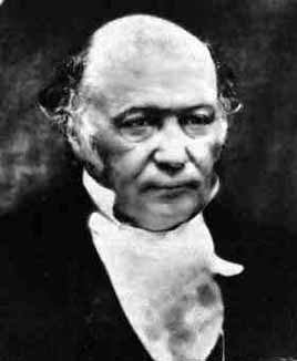
In physics, Hamiltonian mechanics is a reformulation of Lagrangian mechanics that emerged in 1833. Introduced by Sir William Rowan Hamilton, Hamiltonian mechanics replaces (generalized) velocities used in Lagrangian mechanics with (generalized) momenta. Both theories provide interpretations of classical mechanics and describe the same physical phenomena.
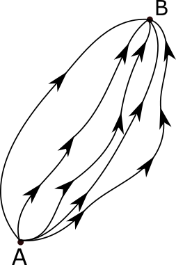
The path integral formulation is a description in quantum mechanics that generalizes the stationary action principle of classical mechanics. It replaces the classical notion of a single, unique classical trajectory for a system with a sum, or functional integral, over an infinity of quantum-mechanically possible trajectories to compute a quantum amplitude.
Geometrical optics, or ray optics, is a model of optics that describes light propagation in terms of rays. The ray in geometrical optics is an abstraction useful for approximating the paths along which light propagates under certain circumstances.

In quantum field theory, the Lehmann–Symanzik–Zimmermann (LSZ) reduction formula is a method to calculate S-matrix elements from the time-ordered correlation functions of a quantum field theory. It is a step of the path that starts from the Lagrangian of some quantum field theory and leads to prediction of measurable quantities. It is named after the three German physicists Harry Lehmann, Kurt Symanzik and Wolfhart Zimmermann.
In mathematics and physics, the Christoffel symbols are an array of numbers describing a metric connection. The metric connection is a specialization of the affine connection to surfaces or other manifolds endowed with a metric, allowing distances to be measured on that surface. In differential geometry, an affine connection can be defined without reference to a metric, and many additional concepts follow: parallel transport, covariant derivatives, geodesics, etc. also do not require the concept of a metric. However, when a metric is available, these concepts can be directly tied to the "shape" of the manifold itself; that shape is determined by how the tangent space is attached to the cotangent space by the metric tensor. Abstractly, one would say that the manifold has an associated (orthonormal) frame bundle, with each "frame" being a possible choice of a coordinate frame. An invariant metric implies that the structure group of the frame bundle is the orthogonal group O(p, q). As a result, such a manifold is necessarily a (pseudo-)Riemannian manifold. The Christoffel symbols provide a concrete representation of the connection of (pseudo-)Riemannian geometry in terms of coordinates on the manifold. Additional concepts, such as parallel transport, geodesics, etc. can then be expressed in terms of Christoffel symbols.

In theoretical physics, the (one-dimensional) nonlinear Schrödinger equation (NLSE) is a nonlinear variation of the Schrödinger equation. It is a classical field equation whose principal applications are to the propagation of light in nonlinear optical fibers and planar waveguides and to Bose–Einstein condensates confined to highly anisotropic, cigar-shaped traps, in the mean-field regime. Additionally, the equation appears in the studies of small-amplitude gravity waves on the surface of deep inviscid (zero-viscosity) water; the Langmuir waves in hot plasmas; the propagation of plane-diffracted wave beams in the focusing regions of the ionosphere; the propagation of Davydov's alpha-helix solitons, which are responsible for energy transport along molecular chains; and many others. More generally, the NLSE appears as one of universal equations that describe the evolution of slowly varying packets of quasi-monochromatic waves in weakly nonlinear media that have dispersion. Unlike the linear Schrödinger equation, the NLSE never describes the time evolution of a quantum state. The 1D NLSE is an example of an integrable model.
The Rayleigh–Ritz method is a direct numerical method of approximating eigenvalues, originated in the context of solving physical boundary value problems and named after Lord Rayleigh and Walther Ritz.

The Timoshenko–Ehrenfest beam theory was developed by Stephen Timoshenko and Paul Ehrenfest early in the 20th century. The model takes into account shear deformation and rotational bending effects, making it suitable for describing the behaviour of thick beams, sandwich composite beams, or beams subject to high-frequency excitation when the wavelength approaches the thickness of the beam. The resulting equation is of fourth order but, unlike Euler–Bernoulli beam theory, there is also a second-order partial derivative present. Physically, taking into account the added mechanisms of deformation effectively lowers the stiffness of the beam, while the result is a larger deflection under a static load and lower predicted eigenfrequencies for a given set of boundary conditions. The latter effect is more noticeable for higher frequencies as the wavelength becomes shorter, and thus the distance between opposing shear forces decreases.

In fluid dynamics, the mild-slope equation describes the combined effects of diffraction and refraction for water waves propagating over bathymetry and due to lateral boundaries—like breakwaters and coastlines. It is an approximate model, deriving its name from being originally developed for wave propagation over mild slopes of the sea floor. The mild-slope equation is often used in coastal engineering to compute the wave-field changes near harbours and coasts.
In the finite element method for the numerical solution of elliptic partial differential equations, the stiffness matrix is a matrix that represents the system of linear equations that must be solved in order to ascertain an approximate solution to the differential equation.
In mathematics, the method of steepest descent or saddle-point method is an extension of Laplace's method for approximating an integral, where one deforms a contour integral in the complex plane to pass near a stationary point, in roughly the direction of steepest descent or stationary phase. The saddle-point approximation is used with integrals in the complex plane, whereas Laplace’s method is used with real integrals.
Curvilinear coordinates can be formulated in tensor calculus, with important applications in physics and engineering, particularly for describing transportation of physical quantities and deformation of matter in fluid mechanics and continuum mechanics.
Lagrangian field theory is a formalism in classical field theory. It is the field-theoretic analogue of Lagrangian mechanics. Lagrangian mechanics is used to analyze the motion of a system of discrete particles each with a finite number of degrees of freedom. Lagrangian field theory applies to continua and fields, which have an infinite number of degrees of freedom.

In numerical mathematics, the gradient discretisation method (GDM) is a framework which contains classical and recent numerical schemes for diffusion problems of various kinds: linear or non-linear, steady-state or time-dependent. The schemes may be conforming or non-conforming, and may rely on very general polygonal or polyhedral meshes.


