Continuity equation

A continuity equation or transport equation is an equation that describes the transport of some quantity. It is particularly simple and powerful when applied to a conserved quantity, but it can be generalized to apply to any extensive quantity. Since mass, energy, momentum, electric charge and other natural quantities are conserved under their respective appropriate conditions, a variety of physical phenomena may be described using continuity equations.

Continuity equations are a stronger, local form of conservation laws. For example, a weak version of the law of conservation of energy states that energy can neither be created nor destroyed—i.e., the total amount of energy in the universe is fixed. This statement does not rule out the possibility that a quantity of energy could disappear from one point while simultaneously appearing at another point. A stronger statement is that energy is locally conserved: energy can neither be created nor destroyed, nor can it "teleport" from one place to another—it can only move by a continuous flow. A continuity equation is the mathematical way to express this kind of statement. For example, the continuity equation for electric charge states that the amount of electric charge in any volume of space can only change by the amount of electric current flowing into or out of that volume through its boundaries.

Continuity equations more generally can include "source" and "sink" terms, which allow them to describe quantities that are often but not always conserved, such as the density of a molecular species which can be created or destroyed by chemical reactions. In an everyday example, there is a continuity equation for the number of people alive; it has a "source term" to account for people being born, and a "sink term" to account for people dying.

Any continuity equation can be expressed in an "integral form" (in terms of a flux integral), which applies to any finite region, or in a "differential form" (in terms of the divergence operator) which applies at a point.

Continuity equations underlie more specific transport equations such as the convection–diffusion equation, Boltzmann transport equation, and Navier–Stokes equations.

Flows governed by continuity equations can be visualized using a Sankey diagram.

General equation

Definition of flux

Main article: Flux

A continuity equation is useful when a flux can be defined. To define flux, first there must be a quantity q which can flow or move, such as mass, energy, electric charge, momentum, number of molecules, etc. Let ρ be the volume density of this quantity, that is, the amount of q per unit volume.

The way that this quantity q is flowing is described by its flux. The flux of q is a vector field, which we denote as j. Here are some examples and properties of flux:

• The dimension of flux is "amount of q flowing per unit time, through a unit area". For example, in the mass continuity equation for flowing water, if 1 gram per second of water is flowing through a pipe with cross-sectional area 1 cm², then the average mass flux j inside the pipe is (1 g/s) / cm², and its direction is along the pipe in the direction that the water is flowing. Outside the pipe, where there is no water, the flux is zero.
• If there is a velocity field u which describes the relevant flow—in other words, if all of the quantity q at a point x is moving with velocity u(x)—then the flux is by definition equal to the density times the velocity field:

$${\displaystyle \mathbf {j} =\rho \mathbf {u} }$$

For example, if in the mass continuity equation for flowing water, u is the water's velocity at each point, and ρ is the water's density at each point, then j would be the mass flux, also known as the material discharge.

• In a well-known example, the flux of electric charge is the electric current density.

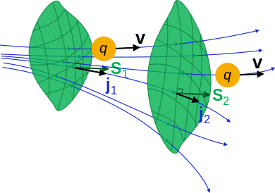
Illustration of how the fluxes, or flux densities, j₁ and j₂ of a quantity q pass through open surfaces S₁ and S₂. (vectors S₁ and S₂ represent vector areas that can be differentiated into infinitesimal area elements).

• If there is an imaginary surface S, then the surface integral of flux over S is equal to the amount of q that is passing through the surface S per unit time:

${\displaystyle ({\text{Rate that }}q{\text{ is flowing through the imaginary surface }}S)=\iint _{S}\mathbf {j} \cdot d\mathbf {S} }$

in which ${\textstyle \iint _{S}d\mathbf {S} }$ is a surface integral.

(Note that the concept that is here called "flux" is alternatively termed flux density in some literature, in which context "flux" denotes the surface integral of flux density. See the main article on Flux for details.)

Integral form

The integral form of the continuity equation states that:

• The amount of q in a region increases when additional q flows inward through the surface of the region, and decreases when it flows outward;
• The amount of q in a region increases when new q is created inside the region, and decreases when q is destroyed;
• Apart from these two processes, there is no other way for the amount of q in a region to change.

Mathematically, the integral form of the continuity equation expressing the rate of increase of q within a volume V is:

${\displaystyle {\frac {dq}{dt}}+\oint _{S}\mathbf {j} \cdot d\mathbf {S} =\Sigma }$

In the integral form of the continuity equation, S is any closed surface that fully encloses a volume V, like any of the surfaces on the left. S can not be a surface with boundaries, like those on the right. (Surfaces are blue, boundaries are red.)

where

• S is any imaginary closed surface, that encloses a volume V,
• ${\displaystyle \oint _{S}d\mathbf {S} }$ denotes a surface integral over that closed surface,
• q is the total amount of the quantity in the volume V,
• j is the flux of q,
• t is time,
• Σ is the net rate that q is being generated inside the volume V per unit time. When q is being generated, it is called a source of q, and it makes Σ more positive. When q is being destroyed, it is called a sink of q, and it makes Σ more negative. This term is sometimes written as ${\displaystyle dq/dt|_{\text{gen}}}$ or the total change of q from its generation or destruction inside the control volume.

In a simple example, V could be a building, and q could be the number of people in the building. The surface S would consist of the walls, doors, roof, and foundation of the building. Then the continuity equation states that the number of people in the building increases when people enter the building (an inward flux through the surface), decreases when people exit the building (an outward flux through the surface), increases when someone in the building gives birth (a source, Σ > 0), and decreases when someone in the building dies (a sink, Σ < 0).

Differential form

See also: Conservation law and conservation form

By the divergence theorem, a general continuity equation can also be written in a "differential form":

${\displaystyle {\frac {\partial \rho }{\partial t}}+\nabla \cdot \mathbf {j} =\sigma }$

where

• ∇⋅ is divergence,
• ρ is the density of the amount q (i.e. the quantity q per unit volume),
• j is the flux density of q (i.e. j = ρv, where v is the vector field describing the movement of the quantity q),
• t is time,
• σ is the generation of q per unit volume per unit time. Terms that generate q (i.e., σ > 0) or remove q (i.e., σ < 0) are referred to as a sources and sinks respectively.

This general equation may be used to derive any continuity equation, ranging from as simple as the volume continuity equation to as complicated as the Navier–Stokes equations. This equation also generalizes the advection equation. Other equations in physics, such as Gauss's law of the electric field and Gauss's law for gravity, have a similar mathematical form to the continuity equation, but are not usually referred to by the term "continuity equation", because j in those cases does not represent the flow of a real physical quantity.

In the case that q is a conserved quantity that cannot be created or destroyed (such as energy), σ = 0 and the equations become: $${\displaystyle {\frac {\partial \rho }{\partial t}}+\nabla \cdot \mathbf {j} =0}$$

Electromagnetism

Main article: Charge conservation

In electromagnetic theory, the continuity equation is an empirical law expressing (local) charge conservation. Mathematically it is an automatic consequence of Maxwell's equations, although charge conservation is more fundamental than Maxwell's equations. It states that the divergence of the current density J (in amperes per square meter) is equal to the negative rate of change of the charge density ρ (in coulombs per cubic meter), $${\displaystyle \nabla \cdot \mathbf {J} =-{\frac {\partial \rho }{\partial t}}}$$

Consistency with Maxwell's equations

One of Maxwell's equations, Ampère's law (with Maxwell's correction), states that $${\displaystyle \nabla \times \mathbf {H} =\mathbf {J} +{\frac {\partial \mathbf {D} }{\partial t}}.}$$

Taking the divergence of both sides (the divergence and partial derivative in time commute) results in $${\displaystyle \nabla \cdot (\nabla \times \mathbf {H} )=\nabla \cdot \mathbf {J} +{\frac {\partial (\nabla \cdot \mathbf {D} )}{\partial t}},}$$ but the divergence of a curl is zero, so that $${\displaystyle \nabla \cdot \mathbf {J} +{\frac {\partial (\nabla \cdot \mathbf {D} )}{\partial t}}=0.}$$

But Gauss's law (another Maxwell equation), states that $${\displaystyle \nabla \cdot \mathbf {D} =\rho ,}$$ which can be substituted in the previous equation to yield the continuity equation $${\displaystyle \nabla \cdot \mathbf {J} +{\frac {\partial \rho }{\partial t}}=0.}$$

Current is the movement of charge. The continuity equation says that if charge is moving out of a differential volume (i.e., divergence of current density is positive) then the amount of charge within that volume is going to decrease, so the rate of change of charge density is negative. Therefore, the continuity equation amounts to a conservation of charge.

If magnetic monopoles exist, there would be a continuity equation for monopole currents as well, see the monopole article for background and the duality between electric and magnetic currents.

Fluid dynamics

See also: Mass flux, Mass flow rate, and Vorticity equation

In fluid dynamics, the continuity equation states that the rate at which mass enters a system is equal to the rate at which mass leaves the system plus the accumulation of mass within the system. ^{[1] [2]} The differential form of the continuity equation is: ^[1] $${\displaystyle {\frac {\partial \rho }{\partial t}}+\nabla \cdot (\rho \mathbf {u} )=0}$$ where

• ρ is fluid density,
• t is time,
• u is the flow velocity vector field.

The time derivative can be understood as the accumulation (or loss) of mass in the system, while the divergence term represents the difference in flow in versus flow out. In this context, this equation is also one of the Euler equations (fluid dynamics). The Navier–Stokes equations form a vector continuity equation describing the conservation of linear momentum.

If the fluid is incompressible (volumetric strain rate is zero), the mass continuity equation simplifies to a volume continuity equation: ^[3] $${\displaystyle \nabla \cdot \mathbf {u} =0,}$$ which means that the divergence of the velocity field is zero everywhere. Physically, this is equivalent to saying that the local volume dilation rate is zero, hence a flow of water through a converging pipe will adjust solely by increasing its velocity as water is largely incompressible.

Computer vision

Main article: Optical flow

In computer vision, optical flow is the pattern of apparent motion of objects in a visual scene. Under the assumption that brightness of the moving object did not change between two image frames, one can derive the optical flow equation as:^{[ citation needed ]}$${\displaystyle {\frac {\partial I}{\partial x}}V_{x}+{\frac {\partial I}{\partial y}}V_{y}+{\frac {\partial I}{\partial t}}=\nabla I\cdot \mathbf {V} +{\frac {\partial I}{\partial t}}=0}$$ where

• t is time,
• x, y coordinates in the image,
• I is the image intensity at image coordinate (x, y) and time t,
• V is the optical flow velocity vector ${\displaystyle (V_{x},V_{y})}$ at image coordinate (x, y) and time t

Energy and heat

Conservation of energy says that energy cannot be created or destroyed. (See below for the nuances associated with general relativity.) Therefore, there is a continuity equation for energy flow: $${\displaystyle {\frac {\partial u}{\partial t}}+\nabla \cdot \mathbf {q} =0}$$ where

• u, local energy density (energy per unit volume),
• q, energy flux (transfer of energy per unit cross-sectional area per unit time) as a vector,

An important practical example is the flow of heat. When heat flows inside a solid, the continuity equation can be combined with Fourier's law (heat flux is proportional to temperature gradient) to arrive at the heat equation. The equation of heat flow may also have source terms: Although energy cannot be created or destroyed, heat can be created from other types of energy, for example via friction or joule heating.

Probability distributions

If there is a quantity that moves continuously according to a stochastic (random) process, like the location of a single dissolved molecule with Brownian motion, then there is a continuity equation for its probability distribution. The flux in this case is the probability per unit area per unit time that the particle passes through a surface. According to the continuity equation, the negative divergence of this flux equals the rate of change of the probability density. The continuity equation reflects the fact that the molecule is always somewhere—the integral of its probability distribution is always equal to 1—and that it moves by a continuous motion (no teleporting).

Quantum mechanics

Quantum mechanics is another domain where there is a continuity equation related to conservation of probability. The terms in the equation require the following definitions, and are slightly less obvious than the other examples above, so they are outlined here:

• The wavefunction Ψ for a single particle in position space (rather than momentum space), that is, a function of position r and time t, Ψ = Ψ(r, t).
• The probability density function is $${\displaystyle \rho (\mathbf {r} ,t)=\Psi ^{*}(\mathbf {r} ,t)\Psi (\mathbf {r} ,t)=|\Psi (\mathbf {r} ,t)|^{2}.}$$
• The probability of finding the particle within V at t is denoted and defined by $${\displaystyle P=P_{\mathbf {r} \in V}(t)=\int _{V}\Psi ^{*}\Psi dV=\int _{V}|\Psi |^{2}dV.}$$
• The probability current (probability flux) is $${\displaystyle \mathbf {j} (\mathbf {r} ,t)={\frac {\hbar }{2mi}}\left[\Psi ^{*}\left(\nabla \Psi \right)-\Psi \left(\nabla \Psi ^{*}\right)\right].}$$

With these definitions the continuity equation reads: $${\displaystyle \nabla \cdot \mathbf {j} +{\frac {\partial \rho }{\partial t}}=0\mathrel {\rightleftharpoons } \nabla \cdot \mathbf {j} +{\frac {\partial |\Psi |^{2}}{\partial t}}=0.}$$

Either form may be quoted. Intuitively, the above quantities indicate this represents the flow of probability. The chance of finding the particle at some position r and time t flows like a fluid; hence the term probability current, a vector field. The particle itself does not flow deterministically in this vector field.

Consistency with Schrödinger equation

The time dependent Schrödinger equation and its complex conjugate (i → −i throughout) are respectively: ^[4] $${\displaystyle {\begin{aligned}-{\frac {\hbar ^{2}}{2m}}\nabla ^{2}\Psi +U\Psi &=i\hbar {\frac {\partial \Psi }{\partial t}},\\-{\frac {\hbar ^{2}}{2m}}\nabla ^{2}\Psi ^{*}+U\Psi ^{*}&=-i\hbar {\frac {\partial \Psi ^{*}}{\partial t}},\\\end{aligned}}}$$ where U is the potential function. The partial derivative of ρ with respect to t is: $${\displaystyle {\frac {\partial \rho }{\partial t}}={\frac {\partial |\Psi |^{2}}{\partial t}}={\frac {\partial }{\partial t}}\left(\Psi ^{*}\Psi \right)=\Psi ^{*}{\frac {\partial \Psi }{\partial t}}+\Psi {\frac {\partial \Psi ^{*}}{\partial t}}.}$$

Multiplying the Schrödinger equation by Ψ* then solving for Ψ* ⁠∂Ψ/∂t⁠, and similarly multiplying the complex conjugated Schrödinger equation by Ψ then solving for Ψ ⁠∂Ψ*/∂t⁠; $${\displaystyle {\begin{aligned}\Psi ^{*}{\frac {\partial \Psi }{\partial t}}&={\frac {1}{i\hbar }}\left[-{\frac {\hbar ^{2}\Psi ^{*}}{2m}}\nabla ^{2}\Psi +U\Psi ^{*}\Psi \right],\\\Psi {\frac {\partial \Psi ^{*}}{\partial t}}&=-{\frac {1}{i\hbar }}\left[-{\frac {\hbar ^{2}\Psi }{2m}}\nabla ^{2}\Psi ^{*}+U\Psi \Psi ^{*}\right],\\\end{aligned}}}$$

substituting into the time derivative of ρ: $${\displaystyle {\begin{aligned}{\frac {\partial \rho }{\partial t}}&={\frac {1}{i\hbar }}\left[-{\frac {\hbar ^{2}\Psi ^{*}}{2m}}\nabla ^{2}\Psi +U\Psi ^{*}\Psi \right]-{\frac {1}{i\hbar }}\left[-{\frac {\hbar ^{2}\Psi }{2m}}\nabla ^{2}\Psi ^{*}+U\Psi \Psi ^{*}\right]\\&={\frac {1}{i\hbar }}\left[-{\frac {\hbar ^{2}\Psi ^{*}}{2m}}\nabla ^{2}\Psi +U\Psi ^{*}\Psi \right]+{\frac {1}{i\hbar }}\left[+{\frac {\hbar ^{2}\Psi }{2m}}\nabla ^{2}\Psi ^{*}-U\Psi ^{*}\Psi \right]\\[2pt]&=-{\frac {1}{i\hbar }}{\frac {\hbar ^{2}\Psi ^{*}}{2m}}\nabla ^{2}\Psi +{\frac {1}{i\hbar }}{\frac {\hbar ^{2}\Psi }{2m}}\nabla ^{2}\Psi ^{*}\\[2pt]&={\frac {\hbar }{2im}}\left[\Psi \nabla ^{2}\Psi ^{*}-\Psi ^{*}\nabla ^{2}\Psi \right]\\\end{aligned}}}$$

The Laplacian operators (∇²) in the above result suggest that the right hand side is the divergence of j, and the reversed order of terms imply this is the negative of j, altogether: $${\displaystyle {\begin{aligned}\nabla \cdot \mathbf {j} &=\nabla \cdot \left[{\frac {\hbar }{2mi}}\left(\Psi ^{*}\left(\nabla \Psi \right)-\Psi \left(\nabla \Psi ^{*}\right)\right)\right]\\&={\frac {\hbar }{2mi}}\left[\Psi ^{*}\left(\nabla ^{2}\Psi \right)-\Psi \left(\nabla ^{2}\Psi ^{*}\right)\right]\\&=-{\frac {\hbar }{2mi}}\left[\Psi \left(\nabla ^{2}\Psi ^{*}\right)-\Psi ^{*}\left(\nabla ^{2}\Psi \right)\right]\\\end{aligned}}}$$ so the continuity equation is: $${\displaystyle {\begin{aligned}&{\frac {\partial \rho }{\partial t}}=-\nabla \cdot \mathbf {j} \\[3pt]{}\Rightarrow {}&{\frac {\partial \rho }{\partial t}}+\nabla \cdot \mathbf {j} =0\\\end{aligned}}}$$

The integral form follows as for the general equation.

Semiconductor

The total current flow in the semiconductor consists of drift current and diffusion current of both the electrons in the conduction band and holes in the valence band.

General form for electrons in one-dimension: $${\displaystyle {\frac {\partial n}{\partial t}}=n\mu _{n}{\frac {\partial E}{\partial x}}+\mu _{n}E{\frac {\partial n}{\partial x}}+D_{n}{\frac {\partial ^{2}n}{\partial x^{2}}}+(G_{n}-R_{n})}$$ where:

• n is the local concentration of electrons
• ${\displaystyle \mu _{n}}$ is electron mobility
• E is the electric field across the depletion region
• D_n is the diffusion coefficient for electrons
• G_n is the rate of generation of electrons
• R_n is the rate of recombination of electrons

Similarly, for holes: $${\displaystyle {\frac {\partial p}{\partial t}}=-p\mu _{p}{\frac {\partial E}{\partial x}}-\mu _{p}E{\frac {\partial p}{\partial x}}+D_{p}{\frac {\partial ^{2}p}{\partial x^{2}}}+(G_{p}-R_{p})}$$ where:

• p is the local concentration of holes
• ${\displaystyle \mu _{p}}$ is hole mobility
• E is the electric field across the depletion region
• D_p is the diffusion coefficient for holes
• G_p is the rate of generation of holes
• R_p is the rate of recombination of holes

Derivation

This section presents a derivation of the equation above for electrons. A similar derivation can be found for the equation for holes.

Consider the fact that the number of electrons is conserved across a volume of semiconductor material with cross-sectional area, A, and length, dx, along the x-axis. More precisely, one can say: $${\displaystyle {\text{Rate of change of electron density}}=({\text{Electron flux in}}-{\text{Electron flux out}})+{\text{Net generation inside a volume}}}$$

Mathematically, this equality can be written: $${\displaystyle {\begin{aligned}{\frac {dn}{dt}}A\,dx&=\left[J(x+dx)-J(x)\right]{\frac {A}{e}}+(G_{n}-R_{n})A\,dx\\&=\left[J(x)+{\frac {dJ}{dx}}dx-J(x)\right]{\frac {A}{e}}+(G_{n}-R_{n})A\,dx\\[1.2ex]{\frac {dn}{dt}}&={\frac {1}{e}}{\frac {dJ}{dx}}+(G_{n}-R_{n})\end{aligned}}}$$Here J denotes current density(whose direction is against electron flow by convention) due to electron flow within the considered volume of the semiconductor. It is also called electron current density.

Total electron current density is the sum of drift current and diffusion current densities: $${\displaystyle J_{n}=en\mu _{n}E+eD_{n}{\frac {dn}{dx}}}$$

Therefore, we have $${\displaystyle {\frac {dn}{dt}}={\frac {1}{e}}{\frac {d}{dx}}\left(en\mu _{n}E+eD_{n}{\frac {dn}{dx}}\right)+(G_{n}-R_{n})}$$

Applying the product rule results in the final expression: $${\displaystyle {\frac {dn}{dt}}=\mu _{n}E{\frac {dn}{dx}}+\mu _{n}n{\frac {dE}{dx}}+D_{n}{\frac {d^{2}n}{dx^{2}}}+(G_{n}-R_{n})}$$

Solution

The key to solving these equations in real devices is whenever possible to select regions in which most of the mechanisms are negligible so that the equations reduce to a much simpler form.

Relativistic version

Special relativity

See also: 4-vector

The notation and tools of special relativity, especially 4-vectors and 4-gradients, offer a convenient way to write any continuity equation.

The density of a quantity ρ and its current j can be combined into a 4-vector called a 4-current: $${\displaystyle J=\left(c\rho ,j_{x},j_{y},j_{z}\right)}$$ where c is the speed of light. The 4-divergence of this current is: $${\displaystyle \partial _{\mu }J^{\mu }=c{\frac {\partial \rho }{\partial ct}}+\nabla \cdot \mathbf {j} }$$ where ∂_μ is the 4-gradient and μ is an index labeling the spacetime dimension. Then the continuity equation is: $${\displaystyle \partial _{\mu }J^{\mu }=0}$$ in the usual case where there are no sources or sinks, that is, for perfectly conserved quantities like energy or charge. This continuity equation is manifestly ("obviously") Lorentz invariant.

Examples of continuity equations often written in this form include electric charge conservation $${\displaystyle \partial _{\mu }J^{\mu }=0}$$ where J is the electric 4-current; and energy–momentum conservation $${\displaystyle \partial _{\nu }T^{\mu \nu }=0}$$ where T is the stress–energy tensor.

General relativity

In general relativity, where spacetime is curved, the continuity equation (in differential form) for energy, charge, or other conserved quantities involves the covariant divergence instead of the ordinary divergence.

For example, the stress–energy tensor is a second-order tensor field containing energy–momentum densities, energy–momentum fluxes, and shear stresses, of a mass-energy distribution. The differential form of energy–momentum conservation in general relativity states that the covariant divergence of the stress-energy tensor is zero: $${\displaystyle {T^{\mu }}_{\nu$$ ;\mu }=0.}

This is an important constraint on the form the Einstein field equations take in general relativity. ^[5]

However, the ordinary divergence of the stress–energy tensor does not necessarily vanish: ^[6] $${\displaystyle \partial _{\mu }T^{\mu \nu }=-\Gamma _{\mu \lambda }^{\mu }T^{\lambda \nu }-\Gamma _{\mu \lambda }^{\nu }T^{\mu \lambda },}$$

The right-hand side strictly vanishes for a flat geometry only.

As a consequence, the integral form of the continuity equation is difficult to define and not necessarily valid for a region within which spacetime is significantly curved (e.g. around a black hole, or across the whole universe). ^[7]

Particle physics

Quarks and gluons have color charge , which is always conserved like electric charge, and there is a continuity equation for such color charge currents (explicit expressions for currents are given at gluon field strength tensor).

There are many other quantities in particle physics which are often or always conserved: baryon number (proportional to the number of quarks minus the number of antiquarks), electron number, mu number, tau number, isospin, and others. ^[8] Each of these has a corresponding continuity equation, possibly including source / sink terms.

Noether's theorem

For more detailed explanations and derivations, see Noether's theorem.

One reason that conservation equations frequently occur in physics is Noether's theorem. This states that whenever the laws of physics have a continuous symmetry, there is a continuity equation for some conserved physical quantity. The three most famous examples are:

• The laws of physics are invariant with respect to time-translation—for example, the laws of physics today are the same as they were yesterday. This symmetry leads to the continuity equation for conservation of energy.
• The laws of physics are invariant with respect to space-translation—for example, a rocket in outer space is not subject to different forces or potentials if it is displaced in any given direction (eg. x, y, z), leading to the conservation of the three components of momentum conservation of momentum.
• The laws of physics are invariant with respect to orientation—for example, floating in outer space, there is no measurement you can do to say "which way is up"; the laws of physics are the same regardless of how you are oriented. This symmetry leads to the continuity equation for conservation of angular momentum.

See also

• Conservation law
• Conservation form
• Dissipative system

References

1. Pedlosky, Joseph (1987). Geophysical fluid dynamics. Springer. pp.  10–13. ISBN   978-0-387-96387-7.
2. Clancy, L.J.(1975), Aerodynamics, Section 3.3, Pitman Publishing Limited, London
3. Fielding, Suzanne. "The Basics of Fluid Dynamics" (PDF). Durham University. Retrieved 22 December 2019.
4. For this derivation see for example McMahon, D. (2006). Quantum Mechanics Demystified. McGraw Hill. ISBN   0-07-145546-9.
5. D. McMahon (2006). Relativity DeMystified. McGraw Hill (USA). ISBN   0-07-145545-0.
6. C.W. Misner; K.S. Thorne; J.A. Wheeler (1973). Gravitation. W.H. Freeman & Co. ISBN   0-7167-0344-0.
7. Michael Weiss; John Baez. "Is Energy Conserved in General Relativity?" . Retrieved 2014-04-25.
8. C.W. Misner; K.S. Thorne; J.A. Wheeler (1973). Gravitation. W.H. Freeman & Co. pp. 558–559. ISBN   0-7167-0344-0.

Further reading

• Lamb, H. (2006) [1932]. Hydrodynamics (6th ed.). Cambridge University Press. ISBN   978-0-521-45868-9.
• Griffiths, D. J. (1999). Introduction to Electrodynamics (3rd ed.). Pearson Education Inc. ISBN   81-7758-293-3.
• Grant, I. S.; Phillips, W. R. (2008). Electromagnetism. Manchester Physics Series (2nd ed.). ISBN   978-0-471-92712-9.
• Wheeler, J. A.; Misner, C.; Thorne, K. S. (1973). Gravitation . W. H. Freeman & Co. ISBN   0-7167-0344-0.