Index notation

Last updated October 30, 2023

In mathematics and computer programming, index notation is used to specify the elements of an array of numbers. The formalism of how indices are used varies according to the subject. In particular, there are different methods for referring to the elements of a list, a vector, or a matrix, depending on whether one is writing a formal mathematical paper for publication, or when one is writing a computer program.

In mathematics

It is frequently helpful in mathematics to refer to the elements of an array using subscripts. The subscripts can be integers or variables. The array takes the form of tensors in general, since these can be treated as multi-dimensional arrays. Special (and more familiar) cases are vectors (1d arrays) and matrices (2d arrays).

The following is only an introduction to the concept: index notation is used in more detail in mathematics (particularly in the representation and manipulation of tensor operations). See the main article for further details.

One-dimensional arrays (vectors)

A vector treated as an array of numbers by writing as a row vector or column vector (whichever is used depends on convenience or context):

\mathbf {a} ={\begin{pmatrix}a_{1}\\a_{2}\\\vdots \\a_{n}\end{pmatrix}},\quad \mathbf {a} ={\begin{pmatrix}a_{1}&a_{2}&\cdots &a_{n}\end{pmatrix}}

Index notation allows indication of the elements of the array by simply writing a_i, where the index i is known to run from 1 to n, because of n-dimensions.^[1] For example, given the vector:

\mathbf {a} ={\begin{pmatrix}10&8&9&6&3&5\\\end{pmatrix}}

then some entries are

a_{1}=10,\,a_{2}=8,\,\cdots ,\,a_{6}=5

.

The notation can be applied to vectors in mathematics and physics. The following vector equation

\mathbf {a} +\mathbf {b} =\mathbf {c}

can also be written in terms of the elements of the vector (aka components), that is

a_{i}+b_{i}=c_{i}

where the indices take a given range of values. This expression represents a set of equations, one for each index. If the vectors each have n elements, meaning i = 1,2,…n, then the equations are explicitly

{\begin{aligned}a_{1}+b_{1}&=c_{1}\\a_{2}+b_{2}&=c_{2}\\&\ \ \vdots \\a_{n}+b_{n}&=c_{n}\end{aligned}}

Hence, index notation serves as an efficient shorthand for

representing the general structure to an equation,
while applicable to individual components.

Two-dimensional arrays

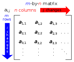
Elements of matrix A are described with two subscripts or indices. Matrix.svg — Elements of matrix A are described with two subscripts or indices.

More than one index is used to describe arrays of numbers, in two or more dimensions, such as the elements of a matrix, (see also image to right);

\mathbf {A} ={\begin{pmatrix}a_{11}&a_{12}&\cdots &a_{1n}\\a_{21}&a_{22}&\cdots &a_{2n}\\\vdots &\vdots &\ddots &\vdots \\a_{m1}&a_{m2}&\cdots &a_{mn}\\\end{pmatrix}}

The entry of a matrix A is written using two indices, say i and j, with or without commas to separate the indices: a_ij or a_i,j, where the first subscript is the row number and the second is the column number. Juxtaposition is also used as notation for multiplication; this may be a source of confusion. For example, if

\mathbf {A} ={\begin{pmatrix}9&8&6\\1&2&7\\4&9&2\\6&0&5\end{pmatrix}}

then some entries are

a_{11}=9,\,a_{12}=8,\,a_{21}=1,\,\cdots ,\,a_{23}=7,\,\cdots

.

For indices larger than 9, the comma-based notation may be preferable (e.g., a_3,12 instead of a₃₁₂).

Matrix equations are written similarly to vector equations, such as

\mathbf {A} +\mathbf {B} =\mathbf {C}

in terms of the elements of the matrices (aka components)

A_{ij}+B_{ij}=C_{ij}

for all values of i and j. Again this expression represents a set of equations, one for each index. If the matrices each have m rows and n columns, meaning i = 1, 2, …, m and j = 1, 2, …, n, then there are mn equations.

Multi-dimensional arrays

The notation allows a clear generalization to multi-dimensional arrays of elements: tensors. For example,

A_{i_{1}i_{2}\cdots }+B_{i_{1}i_{2}\cdots }=C_{i_{1}i_{2}\cdots }

representing a set of many equations.

In tensor analysis, superscripts are used instead of subscripts to distinguish covariant from contravariant entities, see covariance and contravariance of vectors and raising and lowering indices.

In computing

In several programming languages, index notation is a way of addressing elements of an array. This method is used since it is closest to how it is implemented in assembly language whereby the address of the first element is used as a base, and a multiple (the index) of the element size is used to address inside the array.

For example, if an array of integers is stored in a region of the computer's memory starting at the memory cell with address 3000 (the base address), and each integer occupies four cells (bytes), then the elements of this array are at memory locations 0x3000, 0x3004, 0x3008, …, 0x3000 + 4(n − 1) (note the zero-based numbering). In general, the address of the ith element of an array with base address b and element size s is b + is.

Implementation details

In the C programming language, we can write the above as *(base + i) (pointer form) or base[i] (array indexing form), which is exactly equivalent because the C standard defines the array indexing form as a transformation to pointer form. Coincidentally, since pointer addition is commutative, this allows for obscure expressions such as 3[base] which is equivalent to base[3].^[2]

Multidimensional arrays

Things become more interesting when we consider arrays with more than one index, for example, a two-dimensional table. We have three possibilities:

make the two-dimensional array one-dimensional by computing a single index from the two
consider a one-dimensional array where each element is another one-dimensional array, i.e. an array of arrays
use additional storage to hold the array of addresses of each row of the original array, and store the rows of the original array as separate one-dimensional arrays

In C, all three methods can be used. When the first method is used, the programmer decides how the elements of the array are laid out in the computer's memory, and provides the formulas to compute the location of each element. The second method is used when the number of elements in each row is the same and known at the time the program is written. The programmer declares the array to have, say, three columns by writing e.g. elementtype tablename[][3];. One then refers to a particular element of the array by writing tablename[first index][second index]. The compiler computes the total number of memory cells occupied by each row, uses the first index to find the address of the desired row, and then uses the second index to find the address of the desired element in the row. When the third method is used, the programmer declares the table to be an array of pointers, like in elementtype *tablename[];. When the programmer subsequently specifies a particular element tablename[first index][second index], the compiler generates instructions to look up the address of the row specified by the first index, and use this address as the base when computing the address of the element specified by the second index.

voidmult3x3f(floatresult[][3],constfloatA[][3],constfloatB[][3]){inti,j,k;for(i=0;i<3;++i){for(j=0;j<3;++j){result[i][j]=0;for(k=0;k<3;++k)result[i][j]+=A[i][k]*B[k][j];}}}

In other languages

In other programming languages such as Pascal, indices may start at 1, so indexing in a block of memory can be changed to fit a start-at-1 addressing scheme by a simple linear transformation – in this scheme, the memory location of the ith element with base address b and element size s is b + (i − 1)s.

Related Research Articles

Bra–ket notation, also called Dirac notation, is a notation for linear algebra and linear operators on complex vector spaces together with their dual space both in the finite-dimensional and infinite-dimensional case. It is specifically designed to ease the types of calculations that frequently come up in quantum mechanics. Its use in quantum mechanics is quite widespread.

In mathematics, the determinant is a scalar value that is a function of the entries of a square matrix. The determinant of a matrix $A$ is commonly denoted $det(A)$ , $det A$ , or $| A |$ . Its value characterizes some properties of the matrix and the linear map represented by the matrix. In particular, the determinant is nonzero if and only if the matrix is invertible and the linear map represented by the matrix is an isomorphism. The determinant of a product of matrices is the product of their determinants (which follows directly from the above properties).

In mathematics, and more specifically in linear algebra, a linear map is a mapping $between two vector spaces that preserves the operations of vector addition and scalar multiplication. The same names and the same definition are also used for the more general case of modules over a ring; see Module homomorphism.$

In linear algebra, the outer product of two coordinate vectors is the matrix whose entries are all products of an element in the first vector with an element in the second vector. If the two coordinate vectors have dimensions n and m, then their outer product is an n × m matrix. More generally, given two tensors, their outer product is a tensor. The outer product of tensors is also referred to as their tensor product, and can be used to define the tensor algebra.

In mathematics, particularly in linear algebra, matrix multiplication is a binary operation that produces a matrix from two matrices. For matrix multiplication, the number of columns in the first matrix must be equal to the number of rows in the second matrix. The resulting matrix, known as the matrix product, has the number of rows of the first and the number of columns of the second matrix. The product of matrices $A$ and $B$ is denoted as $AB$ .

In mathematics, the cross product or vector product is a binary operation on two vectors in a three-dimensional oriented Euclidean vector space, and is denoted by the symbol $. Given two linearly independent vectors a and b, the cross product, a \times b, is a vector that is perpendicular to both a and b, and thus normal to the plane containing them. The units of the cross-product are the product of the units of each vector. It has many applications in mathematics, physics, engineering, and computer programming. It should not be confused with the dot product.$

In mathematics, especially the usage of linear algebra in mathematical physics, Einstein notation is a notational convention that implies summation over a set of indexed terms in a formula, thus achieving brevity. As part of mathematics it is a notational subset of Ricci calculus; however, it is often used in physics applications that do not distinguish between tangent and cotangent spaces. It was introduced to physics by Albert Einstein in 1916.

In mathematics, particularly in linear algebra, tensor analysis, and differential geometry, the Levi-Civita symbol or Levi-Civita epsilon represents a collection of numbers; defined from the sign of a permutation of the natural numbers $1, 2, ..., n$ , for some positive integer $n$ . It is named after the Italian mathematician and physicist Tullio Levi-Civita. Other names include the permutation symbol, antisymmetric symbol, or alternating symbol, which refer to its antisymmetric property and definition in terms of permutations.

In special relativity, a four-vector is an object with four components, which transform in a specific way under Lorentz transformations. Specifically, a four-vector is an element of a four-dimensional vector space considered as a representation space of the standard representation of the Lorentz group, the representation. It differs from a Euclidean vector in how its magnitude is determined. The transformations that preserve this magnitude are the Lorentz transformations, which include spatial rotations and boosts.

In linear algebra, a minor of a matrix A is the determinant of some smaller square matrix, cut down from A by removing one or more of its rows and columns. Minors obtained by removing just one row and one column from square matrices are required for calculating matrix cofactors, which in turn are useful for computing both the determinant and inverse of square matrices. The requirement that the square matrix be smaller than the original matrix is often omitted in the definition.

In numerical analysis and scientific computing, a sparse matrix or sparse array is a matrix in which most of the elements are zero. There is no strict definition regarding the proportion of zero-value elements for a matrix to qualify as sparse but a common criterion is that the number of non-zero elements is roughly equal to the number of rows or columns. By contrast, if most of the elements are non-zero, the matrix is considered dense. The number of zero-valued elements divided by the total number of elements is sometimes referred to as the sparsity of the matrix.

In mathematics, a block matrix or a partitioned matrix is a matrix that is interpreted as having been broken into sections called blocks or submatrices. Intuitively, a matrix interpreted as a block matrix can be visualized as the original matrix with a collection of horizontal and vertical lines, which break it up, or partition it, into a collection of smaller matrices. Any matrix may be interpreted as a block matrix in one or more ways, with each interpretation defined by how its rows and columns are partitioned.

In mathematics, the Kronecker product, sometimes denoted by ⊗, is an operation on two matrices of arbitrary size resulting in a block matrix. It is a specialization of the tensor product from vectors to matrices and gives the matrix of the tensor product linear map with respect to a standard choice of basis. The Kronecker product is to be distinguished from the usual matrix multiplication, which is an entirely different operation. The Kronecker product is also sometimes called matrix direct product.

In geometry, the line element or length element can be informally thought of as a line segment associated with an infinitesimal displacement vector in a metric space. The length of the line element, which may be thought of as a differential arc length, is a function of the metric tensor and is denoted by .

In mathematics and physics, the Christoffel symbols are an array of numbers describing a metric connection. The metric connection is a specialization of the affine connection to surfaces or other manifolds endowed with a metric, allowing distances to be measured on that surface. In differential geometry, an affine connection can be defined without reference to a metric, and many additional concepts follow: parallel transport, covariant derivatives, geodesics, etc. also do not require the concept of a metric. However, when a metric is available, these concepts can be directly tied to the "shape" of the manifold itself; that shape is determined by how the tangent space is attached to the cotangent space by the metric tensor. Abstractly, one would say that the manifold has an associated (orthonormal) frame bundle, with each "frame" being a possible choice of a coordinate frame. An invariant metric implies that the structure group of the frame bundle is the orthogonal group $O(p, q)$ . As a result, such a manifold is necessarily a (pseudo-)Riemannian manifold. The Christoffel symbols provide a concrete representation of the connection of (pseudo-)Riemannian geometry in terms of coordinates on the manifold. Additional concepts, such as parallel transport, geodesics, etc. can then be expressed in terms of Christoffel symbols.

In geometry and linear algebra, a Cartesian tensor uses an orthonormal basis to represent a tensor in a Euclidean space in the form of components. Converting a tensor's components from one such basis to another is done through an orthogonal transformation.

In numerical analysis and linear algebra, lower–upper (LU) decomposition or factorization factors a matrix as the product of a lower triangular matrix and an upper triangular matrix. The product sometimes includes a permutation matrix as well. LU decomposition can be viewed as the matrix form of Gaussian elimination. Computers usually solve square systems of linear equations using LU decomposition, and it is also a key step when inverting a matrix or computing the determinant of a matrix. The LU decomposition was introduced by the Polish astronomer Tadeusz Banachiewicz in 1938. To quote: "It appears that Gauss and Doolittle applied the method [of elimination] only to symmetric equations. More recent authors, for example, Aitken, Banachiewicz, Dwyer, and Crout … have emphasized the use of the method, or variations of it, in connection with non-symmetric problems … Banachiewicz … saw the point … that the basic problem is really one of matrix factorization, or “decomposition” as he called it." It's also referred to as LR decomposition.

In mathematics, specifically multilinear algebra, a dyadic or dyadic tensor is a second order tensor, written in a notation that fits in with vector algebra.

<span class="mw-page-title-main">Matrix (mathematics)</span> Array of numbers

In mathematics, a matrix is a rectangular array or table of numbers, symbols, or expressions, arranged in rows and columns, which is used to represent a mathematical object or a property of such an object.

Symmetries in quantum mechanics describe features of spacetime and particles which are unchanged under some transformation, in the context of quantum mechanics, relativistic quantum mechanics and quantum field theory, and with applications in the mathematical formulation of the standard model and condensed matter physics. In general, symmetry in physics, invariance, and conservation laws, are fundamentally important constraints for formulating physical theories and models. In practice, they are powerful methods for solving problems and predicting what can happen. While conservation laws do not always give the answer to the problem directly, they form the correct constraints and the first steps to solving a multitude of problems.

References

↑ An introduction to Tensor Analysis: For Engineers and Applied Scientists, J.R. Tyldesley, Longman, 1975, ISBN 0-582-44355-5
↑ Programming with C++, J. Hubbard, Schaum's Outlines, McGraw Hill (USA), 1996, ISBN 0-07-114328-9

Programming with C++, J. Hubbard, Schaum's Outlines, McGraw Hill (USA), 1996, ISBN 0-07-114328-9
Tensor Calculus, D.C. Kay, Schaum's Outlines, McGraw Hill (USA), 1988, ISBN 0-07-033484-6
Mathematical methods for physics and engineering, K.F. Riley, M.P. Hobson, S.J. Bence, Cambridge University Press, 2010, ISBN 978-0-521-86153-3

This page is based on this Wikipedia article
Text is available under the CC BY-SA 4.0 license; additional terms may apply.
Images, videos and audio are available under their respective licenses.

[1] An introduction to Tensor Analysis: For Engineers and Applied Scientists, J.R. Tyldesley, Longman, 1975, ISBN 0-582-44355-5

[2] Programming with C++, J. Hubbard, Schaum's Outlines, McGraw Hill (USA), 1996, ISBN 0-07-114328-9

[1]

[2]