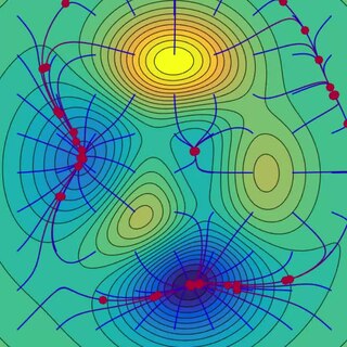
Gradient descent is a method for unconstrained mathematical optimization. It is a first-order iterative algorithm for finding a local minimum of a differentiable multivariate function
In mathematics, and especially differential geometry and gauge theory, a connection on a fiber bundle is a device that defines a notion of parallel transport on the bundle; that is, a way to "connect" or identify fibers over nearby points. The most common case is that of a linear connection on a vector bundle, for which the notion of parallel transport must be linear. A linear connection is equivalently specified by a covariant derivative, an operator that differentiates sections of the bundle along tangent directions in the base manifold, in such a way that parallel sections have derivative zero. Linear connections generalize, to arbitrary vector bundles, the Levi-Civita connection on the tangent bundle of a pseudo-Riemannian manifold, which gives a standard way to differentiate vector fields. Nonlinear connections generalize this concept to bundles whose fibers are not necessarily linear.
In mathematics, a Dirichlet problem is the problem of finding a function which solves a specified partial differential equation (PDE) in the interior of a given region that takes prescribed values on the boundary of the region.
The Newmark-beta method is a method of numerical integration used to solve certain differential equations. It is widely used in numerical evaluation of the dynamic response of structures and solids such as in finite element analysis to model dynamic systems. The method is named after Nathan M. Newmark, former Professor of Civil Engineering at the University of Illinois at Urbana–Champaign, who developed it in 1959 for use in structural dynamics. The semi-discretized structural equation is a second order ordinary differential equation system,
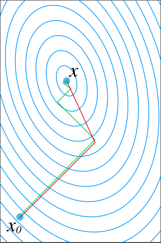
In mathematics, the conjugate gradient method is an algorithm for the numerical solution of particular systems of linear equations, namely those whose matrix is positive-definite. The conjugate gradient method is often implemented as an iterative algorithm, applicable to sparse systems that are too large to be handled by a direct implementation or other direct methods such as the Cholesky decomposition. Large sparse systems often arise when numerically solving partial differential equations or optimization problems.
In mathematics, holomorphic functional calculus is functional calculus with holomorphic functions. That is to say, given a holomorphic function f of a complex argument z and an operator T, the aim is to construct an operator, f(T), which naturally extends the function f from complex argument to operator argument. More precisely, the functional calculus defines a continuous algebra homomorphism from the holomorphic functions on a neighbourhood of the spectrum of T to the bounded operators.
In numerical linear algebra, the method of successive over-relaxation (SOR) is a variant of the Gauss–Seidel method for solving a linear system of equations, resulting in faster convergence. A similar method can be used for any slowly converging iterative process.
In mathematics, preconditioning is the application of a transformation, called the preconditioner, that conditions a given problem into a form that is more suitable for numerical solving methods. Preconditioning is typically related to reducing a condition number of the problem. The preconditioned problem is then usually solved by an iterative method.
Numerical linear algebra, sometimes called applied linear algebra, is the study of how matrix operations can be used to create computer algorithms which efficiently and accurately provide approximate answers to questions in continuous mathematics. It is a subfield of numerical analysis, and a type of linear algebra. Computers use floating-point arithmetic and cannot exactly represent irrational data, so when a computer algorithm is applied to a matrix of data, it can sometimes increase the difference between a number stored in the computer and the true number that it is an approximation of. Numerical linear algebra uses properties of vectors and matrices to develop computer algorithms that minimize the error introduced by the computer, and is also concerned with ensuring that the algorithm is as efficient as possible.
In numerical analysis, BDDC (balancing domain decomposition by constraints) is a domain decomposition method for solving large symmetric, positive definite systems of linear equations that arise from the finite element method. BDDC is used as a preconditioner to the conjugate gradient method. A specific version of BDDC is characterized by the choice of coarse degrees of freedom, which can be values at the corners of the subdomains, or averages over the edges or the faces of the interface between the subdomains. One application of the BDDC preconditioner then combines the solution of local problems on each subdomains with the solution of a global coarse problem with the coarse degrees of freedom as the unknowns. The local problems on different subdomains are completely independent of each other, so the method is suitable for parallel computing. With a proper choice of the coarse degrees of freedom (corners in 2D, corners plus edges or corners plus faces in 3D) and with regular subdomain shapes, the condition number of the method is bounded when increasing the number of subdomains, and it grows only very slowly with the number of elements per subdomain. Thus the number of iterations is bounded in the same way, and the method scales well with the problem size and the number of subdomains.
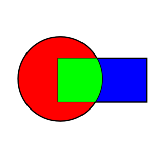
In mathematics, numerical analysis, and numerical partial differential equations, domain decomposition methods solve a boundary value problem by splitting it into smaller boundary value problems on subdomains and iterating to coordinate the solution between adjacent subdomains. A coarse problem with one or few unknowns per subdomain is used to further coordinate the solution between the subdomains globally. The problems on the subdomains are independent, which makes domain decomposition methods suitable for parallel computing. Domain decomposition methods are typically used as preconditioners for Krylov space iterative methods, such as the conjugate gradient method, GMRES, and LOBPCG.
In numerical analysis, the balancing domain decomposition method (BDD) is an iterative method to find the solution of a symmetric positive definite system of linear algebraic equations arising from the finite element method. In each iteration, it combines the solution of local problems on non-overlapping subdomains with a coarse problem created from the subdomain nullspaces. BDD requires only solution of subdomain problems rather than access to the matrices of those problems, so it is applicable to situations where only the solution operators are available, such as in oil reservoir simulation by mixed finite elements. In its original formulation, BDD performs well only for 2nd order problems, such elasticity in 2D and 3D. For 4th order problems, such as plate bending, it needs to be modified by adding to the coarse problem special basis functions that enforce continuity of the solution at subdomain corners, which makes it however more expensive. The BDDC method uses the same corner basis functions as, but in an additive rather than multiplicative fashion. The dual counterpart to BDD is FETI, which enforces the equality of the solution between the subdomain by Lagrange multipliers. The base versions of BDD and FETI are not mathematically equivalent, though a special version of FETI designed to be robust for hard problems has the same eigenvalues and thus essentially the same performance as BDD.
In mathematics, Neumann–Neumann methods are domain decomposition preconditioners named so because they solve a Neumann problem on each subdomain on both sides of the interface between the subdomains. Just like all domain decomposition methods, so that the number of iterations does not grow with the number of subdomains, Neumann–Neumann methods require the solution of a coarse problem to provide global communication. The balancing domain decomposition is a Neumann–Neumann method with a special kind of coarse problem.
In mathematics, a Poincaré–Steklov operator maps the values of one boundary condition of the solution of an elliptic partial differential equation in a domain to the values of another boundary condition. Usually, either of the boundary conditions determines the solution. Thus, a Poincaré–Steklov operator encapsulates the boundary response of the system modelled by the partial differential equation. When the partial differential equation is discretized, for example by finite elements or finite differences, the discretization of the Poincaré–Steklov operator is the Schur complement obtained by eliminating all degrees of freedom inside the domain.
In mathematics, a free boundary problem is a partial differential equation to be solved for both an unknown function and an unknown domain . The segment of the boundary of which is not known at the outset of the problem is the free boundary.
The Kansa method is a computer method used to solve partial differential equations. Its main advantage is it is very easy to understand and program on a computer. It is much less complicated than the finite element method. Another advantage is it works well on multi variable problems. The finite element method is complicated when working with more than 3 space variables and time.
In mathematics, the walk-on-spheres method (WoS) is a numerical probabilistic algorithm, or Monte-Carlo method, used mainly in order to approximate the solutions of some specific boundary value problem for partial differential equations (PDEs). The WoS method was first introduced by Mervin E. Muller in 1956 to solve Laplace's equation, and was since then generalized to other problems.
The Fokas method, or unified transform, is an algorithmic procedure for analysing boundary value problems for linear partial differential equations and for an important class of nonlinear PDEs belonging to the so-called integrable systems. It is named after Greek mathematician Athanassios S. Fokas.
In solid mechanics, the linear stability analysis of an elastic solution is studied using the method of incremental deformations superposed on finite deformations. The method of incremental deformation can be used to solve static, quasi-static and time-dependent problems. The governing equations of the motion are ones of the classical mechanics, such as the conservation of mass and the balance of linear and angular momentum, which provide the equilibrium configuration of the material. The main corresponding mathematical framework is described in the main Raymond Ogden's book Non-linear elastic deformations and in Biot's book Mechanics of incremental deformations, which is a collection of his main papers.
PDE-constrained optimization is a subset of mathematical optimization where at least one of the constraints may be expressed as a partial differential equation. Typical domains where these problems arise include aerodynamics, computational fluid dynamics, image segmentation, and inverse problems. A standard formulation of PDE-constrained optimization encountered in a number of disciplines is given by:


