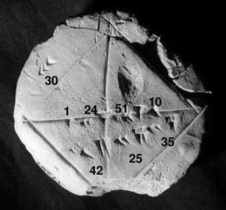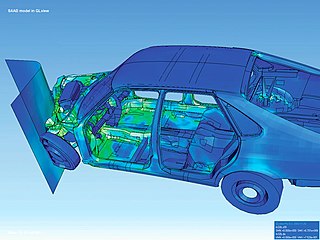
Numerical analysis is the study of algorithms that use numerical approximation for the problems of mathematical analysis. It is the study of numerical methods that attempt to find approximate solutions of problems rather than the exact ones. Numerical analysis finds application in all fields of engineering and the physical sciences, and in the 21st century also the life and social sciences, medicine, business and even the arts. Current growth in computing power has enabled the use of more complex numerical analysis, providing detailed and realistic mathematical models in science and engineering. Examples of numerical analysis include: ordinary differential equations as found in celestial mechanics, numerical linear algebra in data analysis, and stochastic differential equations and Markov chains for simulating living cells in medicine and biology.

In mathematics, a partial differential equation (PDE) is an equation which computes a function between various partial derivatives of a multivariable function.

Numerical methods for ordinary differential equations are methods used to find numerical approximations to the solutions of ordinary differential equations (ODEs). Their use is also known as "numerical integration", although this term can also refer to the computation of integrals.

In mathematics, separation of variables is any of several methods for solving ordinary and partial differential equations, in which algebra allows one to rewrite an equation so that each of two variables occurs on a different side of the equation.
Second-order linear partial differential equations (PDEs) are classified as either elliptic, hyperbolic, or parabolic. Any second-order linear PDE in two variables can be written in the form

In mathematics, a differential equation is an equation that relates one or more unknown functions and their derivatives. In applications, the functions generally represent physical quantities, the derivatives represent their rates of change, and the differential equation defines a relationship between the two. Such relations are common; therefore, differential equations play a prominent role in many disciplines including engineering, physics, economics, and biology.
Numerical methods for partial differential equations is the branch of numerical analysis that studies the numerical solution of partial differential equations (PDEs).
In mathematics, a differential-algebraic system of equations (DAE) is a system of equations that either contains differential equations and algebraic equations, or is equivalent to such a system.

Computational electromagnetics (CEM), computational electrodynamics or electromagnetic modeling is the process of modeling the interaction of electromagnetic fields with physical objects and the environment using computers.
In numerical analysis, finite-difference methods (FDM) are a class of numerical techniques for solving differential equations by approximating derivatives with finite differences. Both the spatial domain and time domain are discretized, or broken into a finite number of intervals, and the values of the solution at the end points of the intervals are approximated by solving algebraic equations containing finite differences and values from nearby points.
A parabolic partial differential equation is a type of partial differential equation (PDE). Parabolic PDEs are used to describe a wide variety of time-dependent phenomena, including heat conduction, particle diffusion, and pricing of derivative investment instruments.
Dynamic simulation is the use of a computer program to model the time-varying behavior of a dynamical system. The systems are typically described by ordinary differential equations or partial differential equations. A simulation run solves the state-equation system to find the behavior of the state variables over a specified period of time. The equation is solved through numerical integration methods to produce the transient behavior of the state variables. Simulation of dynamic systems predicts the values of model-system state variables, as they are determined by the past state values. This relationship is found by creating a model of the system.

The finite element method (FEM) is a popular method for numerically solving differential equations arising in engineering and mathematical modeling. Typical problem areas of interest include the traditional fields of structural analysis, heat transfer, fluid flow, mass transport, and electromagnetic potential.
Finite difference methods for option pricing are numerical methods used in mathematical finance for the valuation of options. Finite difference methods were first applied to option pricing by Eduardo Schwartz in 1977.

In mathematics, an ordinary differential equation (ODE) is a differential equation (DE) dependent on only a single independent variable. As with other DE, its unknown(s) consists of one function(s) and involves the derivatives of those functions. The term "ordinary" is used in contrast with partial differential equations (PDEs) which may be with respect to more than one independent variable, and, less commonly, in contrast with stochastic differential equations (SDEs) where the progression is random.
In mathematics a partial differential algebraic equation (PDAE) set is an incomplete system of partial differential equations that is closed with a set of algebraic equations.

The finite water-content vadose zone flux method represents a one-dimensional alternative to the numerical solution of Richards' equation for simulating the movement of water in unsaturated soils. The finite water-content method solves the advection-like term of the Soil Moisture Velocity Equation, which is an ordinary differential equation alternative to the Richards partial differential equation. The Richards equation is difficult to approximate in general because it does not have a closed-form analytical solution except in a few cases. The finite water-content method, is perhaps the first generic replacement for the numerical solution of the Richards' equation. The finite water-content solution has several advantages over the Richards equation solution. First, as an ordinary differential equation it is explicit, guaranteed to converge and computationally inexpensive to solve. Second, using a finite volume solution methodology it is guaranteed to conserve mass. The finite water content method readily simulates sharp wetting fronts, something that the Richards solution struggles with. The main limiting assumption required to use the finite water-content method is that the soil be homogeneous in layers.
The soil moisture velocity equation describes the speed that water moves vertically through unsaturated soil under the combined actions of gravity and capillarity, a process known as infiltration. The equation is alternative form of the Richardson/Richards' equation. The key difference being that the dependent variable is the position of the wetting front , which is a function of time, the water content and media properties. The soil moisture velocity equation consists of two terms. The first "advection-like" term was developed to simulate surface infiltration and was extended to the water table, which was verified using data collected in a column experimental that was patterned after the famous experiment by Childs & Poulovassilis (1962) and against exact solutions.
Validated numerics, or rigorous computation, verified computation, reliable computation, numerical verification is numerics including mathematically strict error evaluation, and it is one field of numerical analysis. For computation, interval arithmetic is used, and all results are represented by intervals. Validated numerics were used by Warwick Tucker in order to solve the 14th of Smale's problems, and today it is recognized as a powerful tool for the study of dynamical systems.


