Autocorrelation, sometimes known as serial correlation in the discrete time case, is the correlation of a signal with a delayed copy of itself as a function of delay. Informally, it is the similarity between observations of a random variable as a function of the time lag between them. The analysis of autocorrelation is a mathematical tool for finding repeating patterns, such as the presence of a periodic signal obscured by noise, or identifying the missing fundamental frequency in a signal implied by its harmonic frequencies. It is often used in signal processing for analyzing functions or series of values, such as time domain signals.

In mathematics, convolution is a mathematical operation on two functions that produces a third function. The term convolution refers to both the result function and to the process of computing it. It is defined as the integral of the product of the two functions after one is reflected about the y-axis and shifted. The integral is evaluated for all values of shift, producing the convolution function. The choice of which function is reflected and shifted before the integral does not change the integral result. Graphically, it expresses how the 'shape' of one function is modified by the other.

In mathematics, the discrete Fourier transform (DFT) converts a finite sequence of equally-spaced samples of a function into a same-length sequence of equally-spaced samples of the discrete-time Fourier transform (DTFT), which is a complex-valued function of frequency. The interval at which the DTFT is sampled is the reciprocal of the duration of the input sequence. An inverse DFT (IDFT) is a Fourier series, using the DTFT samples as coefficients of complex sinusoids at the corresponding DTFT frequencies. It has the same sample-values as the original input sequence. The DFT is therefore said to be a frequency domain representation of the original input sequence. If the original sequence spans all the non-zero values of a function, its DTFT is continuous, and the DFT provides discrete samples of one cycle. If the original sequence is one cycle of a periodic function, the DFT provides all the non-zero values of one DTFT cycle.

In probability theory, a probability density function (PDF), density function, or density of an absolutely continuous random variable, is a function whose value at any given sample in the sample space can be interpreted as providing a relative likelihood that the value of the random variable would be equal to that sample. Probability density is the probability per unit length, in other words, while the absolute likelihood for a continuous random variable to take on any particular value is 0, the value of the PDF at two different samples can be used to infer, in any particular draw of the random variable, how much more likely it is that the random variable would be close to one sample compared to the other sample.
In mathematics, the Laplace operator or Laplacian is a differential operator given by the divergence of the gradient of a scalar function on Euclidean space. It is usually denoted by the symbols , (where is the nabla operator), or . In a Cartesian coordinate system, the Laplacian is given by the sum of second partial derivatives of the function with respect to each independent variable. In other coordinate systems, such as cylindrical and spherical coordinates, the Laplacian also has a useful form. Informally, the Laplacian Δf (p) of a function f at a point p measures by how much the average value of f over small spheres or balls centered at p deviates from f (p).
In the mathematical field of differential geometry, a metric tensor is an additional structure on a manifold M that allows defining distances and angles, just as the inner product on a Euclidean space allows defining distances and angles there. More precisely, a metric tensor at a point p of M is a bilinear form defined on the tangent space at p, and a metric field on M consists of a metric tensor at each point p of M that varies smoothly with p.
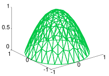
In mathematics, a Gaussian function, often simply referred to as a Gaussian, is a function of the base form and with parametric extension for arbitrary real constants a, b and non-zero c. It is named after the mathematician Carl Friedrich Gauss. The graph of a Gaussian is a characteristic symmetric "bell curve" shape. The parameter a is the height of the curve's peak, b is the position of the center of the peak, and c controls the width of the "bell".

An instanton is a notion appearing in theoretical and mathematical physics. An instanton is a classical solution to equations of motion with a finite, non-zero action, either in quantum mechanics or in quantum field theory. More precisely, it is a solution to the equations of motion of the classical field theory on a Euclidean spacetime.

In condensed matter physics, Bloch's theorem states that solutions to the Schrödinger equation in a periodic potential can be expressed as plane waves modulated by periodic functions. The theorem is named after the Swiss physicist Felix Bloch, who discovered the theorem in 1929. Mathematically, they are written
In mathematics, the Jacobi elliptic functions are a set of basic elliptic functions. They are found in the description of the motion of a pendulum, as well as in the design of electronic elliptic filters. While trigonometric functions are defined with reference to a circle, the Jacobi elliptic functions are a generalization which refer to other conic sections, the ellipse in particular. The relation to trigonometric functions is contained in the notation, for example, by the matching notation for . The Jacobi elliptic functions are used more often in practical problems than the Weierstrass elliptic functions as they do not require notions of complex analysis to be defined and/or understood. They were introduced by Carl Gustav Jakob Jacobi. Carl Friedrich Gauss had already studied special Jacobi elliptic functions in 1797, the lemniscate elliptic functions in particular, but his work was published much later.
In control engineering and system identification, a state-space representation is a mathematical model of a physical system specified as a set of input, output, and variables related by first-order differential equations or difference equations. Such variables, called state variables, evolve over time in a way that depends on the values they have at any given instant and on the externally imposed values of input variables. Output variables’ values depend on the state variable values and may also depend on the input variable values.
In mathematics and signal processing, the Hilbert transform is a specific singular integral that takes a function, u(t) of a real variable and produces another function of a real variable H(u)(t). The Hilbert transform is given by the Cauchy principal value of the convolution with the function (see § Definition). The Hilbert transform has a particularly simple representation in the frequency domain: It imparts a phase shift of ±90° (π/2 radians) to every frequency component of a function, the sign of the shift depending on the sign of the frequency (see § Relationship with the Fourier transform). The Hilbert transform is important in signal processing, where it is a component of the analytic representation of a real-valued signal u(t). The Hilbert transform was first introduced by David Hilbert in this setting, to solve a special case of the Riemann–Hilbert problem for analytic functions.
In mathematics, the matrix exponential is a matrix function on square matrices analogous to the ordinary exponential function. It is used to solve systems of linear differential equations. In the theory of Lie groups, the matrix exponential gives the exponential map between a matrix Lie algebra and the corresponding Lie group.
In signal processing, cross-correlation is a measure of similarity of two series as a function of the displacement of one relative to the other. This is also known as a sliding dot product or sliding inner-product. It is commonly used for searching a long signal for a shorter, known feature. It has applications in pattern recognition, single particle analysis, electron tomography, averaging, cryptanalysis, and neurophysiology. The cross-correlation is similar in nature to the convolution of two functions. In an autocorrelation, which is the cross-correlation of a signal with itself, there will always be a peak at a lag of zero, and its size will be the signal energy.
The Lyapunov equation, named after the Russian mathematician Aleksandr Lyapunov, is a matrix equation used in the stability analysis of linear dynamical systems.
Variational Bayesian methods are a family of techniques for approximating intractable integrals arising in Bayesian inference and machine learning. They are typically used in complex statistical models consisting of observed variables as well as unknown parameters and latent variables, with various sorts of relationships among the three types of random variables, as might be described by a graphical model. As typical in Bayesian inference, the parameters and latent variables are grouped together as "unobserved variables". Variational Bayesian methods are primarily used for two purposes:
- To provide an analytical approximation to the posterior probability of the unobserved variables, in order to do statistical inference over these variables.
- To derive a lower bound for the marginal likelihood of the observed data. This is typically used for performing model selection, the general idea being that a higher marginal likelihood for a given model indicates a better fit of the data by that model and hence a greater probability that the model in question was the one that generated the data.
In probability and statistics, given two stochastic processes and , the cross-covariance is a function that gives the covariance of one process with the other at pairs of time points. With the usual notation for the expectation operator, if the processes have the mean functions and , then the cross-covariance is given by

In algebra, the Bring radical or ultraradical of a real number a is the unique real root of the polynomial
In mathematics – specifically, in stochastic analysis – an Itô diffusion is a solution to a specific type of stochastic differential equation. That equation is similar to the Langevin equation used in physics to describe the Brownian motion of a particle subjected to a potential in a viscous fluid. Itô diffusions are named after the Japanese mathematician Kiyosi Itô.
The streamline upwind Petrov–Galerkin pressure-stabilizing Petrov–Galerkin formulation for incompressible Navier–Stokes equations can be used for finite element computations of high Reynolds number incompressible flow using equal order of finite element space by introducing additional stabilization terms in the Navier–Stokes Galerkin formulation.