Piecewise linear function

Last updated

In mathematics and statistics, a piecewise linear, PL or segmented function is a real-valued function of a real variable, whose graph is composed of straight-line segments. [1]

Contents

Definition

A piecewise linear function is a function defined on a (possibly unbounded) interval of real numbers, such that there is a collection of intervals on each of which the function is an affine function. (Thus "piecewise linear" is actually defined to mean "piecewise affine".) If the domain of the function is compact, there needs to be a finite collection of such intervals; if the domain is not compact, it may either be required to be finite or to be locally finite in the reals.

Examples

A continuous piecewise linear function Piecewise linear function.svg
A continuous piecewise linear function

The function defined by

is piecewise linear with four pieces. The graph of this function is shown to the right. Since the graph of an affine(*) function is a line, the graph of a piecewise linear function consists of line segments and rays. The x values (in the above example −3, 0, and 3) where the slope changes are typically called breakpoints, changepoints, threshold values or knots. As in many applications, this function is also continuous. The graph of a continuous piecewise linear function on a compact interval is a polygonal chain.

Other examples of piecewise linear functions include the absolute value function, the sawtooth function, and the floor function.

(*) A linear function satisfies by definition and therefore in particular ; functions whose graph is a straight line are affine rather than linear.

Fitting to a curve

A function (blue) and a piecewise linear approximation to it (red) Finite element method 1D illustration1.svg
A function (blue) and a piecewise linear approximation to it (red)

An approximation to a known curve can be found by sampling the curve and interpolating linearly between the points. An algorithm for computing the most significant points subject to a given error tolerance has been published. [2]

Fitting to data

If partitions, and then breakpoints, are already known, linear regression can be performed independently on these partitions. However, continuity is not preserved in that case, and also there is no unique reference model underlying the observed data. A stable algorithm with this case has been derived. [3]

If partitions are not known, the residual sum of squares can be used to choose optimal separation points. [4] However efficient computation and joint estimation of all model parameters (including the breakpoints) may be obtained by an iterative procedure [5] currently implemented in the package segmented [6] for the R language.

A variant of decision tree learning called model trees learns piecewise linear functions. [7]

Notation

A piecewise linear function in two dimensions (top) and the convex polytopes on which it is linear (bottom) Piecewise linear function2D.svg
A piecewise linear function in two dimensions (top) and the convex polytopes on which it is linear (bottom)

The notion of a piecewise linear function makes sense in several different contexts. Piecewise linear functions may be defined on n-dimensional Euclidean space, or more generally any vector space or affine space, as well as on piecewise linear manifolds and simplicial complexes (see simplicial map). In each case, the function may be real-valued, or it may take values from a vector space, an affine space, a piecewise linear manifold, or a simplicial complex. (In these contexts, the term “linear” does not refer solely to linear transformations, but to more general affine linear functions.)

In dimensions higher than one, it is common to require the domain of each piece to be a polygon or polytope. This guarantees that the graph of the function will be composed of polygonal or polytopal pieces.

Important sub-classes of piecewise linear functions include the continuous piecewise linear functions and the convex piecewise linear functions. In general, for every n-dimensional continuous piecewise linear function , there is a

such that

[8]

If is convex and continuous, then there is a

such that
Splines generalize piecewise linear functions to higher-order polynomials, which are in turn contained in the category of piecewise-differentiable functions, PDIFF.

Applications

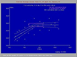
Crop response to depth of the watertable R-3VAR1.JPG
Crop response to depth of the watertable
Example of crop response to soil salinity Mustard segm regr no effect.png
Example of crop response to soil salinity

In agriculture piecewise regression analysis of measured data is used to detect the range over which growth factors affect the yield and the range over which the crop is not sensitive to changes in these factors.

The image on the left shows that at shallow watertables the yield declines, whereas at deeper (> 7 dm) watertables the yield is unaffected. The graph is made using the method of least squares to find the two segments with the best fit.

The graph on the right reveals that crop yields tolerate a soil salinity up to ECe = 8 dS/m (ECe is the electric conductivity of an extract of a saturated soil sample), while beyond that value the crop production reduces. The graph is made with the method of partial regression to find the longest range of "no effect", i.e. where the line is horizontal. The two segments need not join at the same point. Only for the second segment method of least squares is used.

See also

Further reading

Related Research Articles

<span class="mw-page-title-main">Pauli matrices</span> Matrices important in quantum mechanics and the study of spin

In mathematical physics and mathematics, the Pauli matrices are a set of three 2 × 2 complex matrices which are Hermitian, involutory and unitary. Usually indicated by the Greek letter sigma, they are occasionally denoted by tau when used in connection with isospin symmetries.

<span class="mw-page-title-main">Affine transformation</span> Geometric transformation that preserves lines but not angles nor the origin

In Euclidean geometry, an affine transformation or affinity is a geometric transformation that preserves lines and parallelism, but not necessarily Euclidean distances and angles.

In mathematics and in particular measure theory, a measurable function is a function between the underlying sets of two measurable spaces that preserves the structure of the spaces: the preimage of any measurable set is measurable. This is in direct analogy to the definition that a continuous function between topological spaces preserves the topological structure: the preimage of any open set is open. In real analysis, measurable functions are used in the definition of the Lebesgue integral. In probability theory, a measurable function on a probability space is known as a random variable.

In mathematics, a quadric or quadric surface (quadric hypersurface in higher dimensions), is a generalization of conic sections (ellipses, parabolas, and hyperbolas). It is a hypersurface (of dimension D) in a (D + 1)-dimensional space, and it is defined as the zero set of an irreducible polynomial of degree two in D + 1 variables; for example, D = 1 in the case of conic sections. When the defining polynomial is not absolutely irreducible, the zero set is generally not considered a quadric, although it is often called a degenerate quadric or a reducible quadric.

In mathematics, and in particular linear algebra, the Moore–Penrose inverse of a matrix is the most widely known generalization of the inverse matrix. It was independently described by E. H. Moore in 1920, Arne Bjerhammar in 1951, and Roger Penrose in 1955. Earlier, Erik Ivar Fredholm had introduced the concept of a pseudoinverse of integral operators in 1903. When referring to a matrix, the term pseudoinverse, without further specification, is often used to indicate the Moore–Penrose inverse. The term generalized inverse is sometimes used as a synonym for pseudoinverse.

In mathematics, real trees are a class of metric spaces generalising simplicial trees. They arise naturally in many mathematical contexts, in particular geometric group theory and probability theory. They are also the simplest examples of Gromov hyperbolic spaces.

In functional analysis, it is often convenient to define a linear transformation on a complete, normed vector space by first defining a linear transformation on a dense subset of and then continuously extending to the whole space via the theorem below. The resulting extension remains linear and bounded, and is thus continuous, which makes it a continuous linear extension.

In numerical analysis and computational statistics, rejection sampling is a basic technique used to generate observations from a distribution. It is also commonly called the acceptance-rejection method or "accept-reject algorithm" and is a type of exact simulation method. The method works for any distribution in with a density.

<span class="mw-page-title-main">Barycentric subdivision</span>

In mathematics, the barycentric subdivision is a standard way to subdivide a given simplex into smaller ones. Its extension on simplicial complexes is a canonical method to refine them. Therefore, the barycentric subdivision is an important tool in algebraic topology.

<span class="mw-page-title-main">Čech cohomology</span>

In mathematics, specifically algebraic topology, Čech cohomology is a cohomology theory based on the intersection properties of open covers of a topological space. It is named for the mathematician Eduard Čech.

<span class="mw-page-title-main">Triangulation (topology)</span>

In mathematics, triangulation describes the replacement of topological spaces by piecewise linear spaces, i.e. the choice of a homeomorphism in a suitable simplicial complex. Spaces being homeomorphic to a simplicial complex are called triangulable. Triangulation has various uses in different branches of mathematics, for instance in algebraic topology, in complex analysis or in modeling.

Linear discriminant analysis (LDA), normal discriminant analysis (NDA), or discriminant function analysis is a generalization of Fisher's linear discriminant, a method used in statistics and other fields, to find a linear combination of features that characterizes or separates two or more classes of objects or events. The resulting combination may be used as a linear classifier, or, more commonly, for dimensionality reduction before later classification.

Many letters of the Latin alphabet, both capital and small, are used in mathematics, science, and engineering to denote by convention specific or abstracted constants, variables of a certain type, units, multipliers, or physical entities. Certain letters, when combined with special formatting, take on special meaning.

Functional data analysis (FDA) is a branch of statistics that analyses data providing information about curves, surfaces or anything else varying over a continuum. In its most general form, under an FDA framework, each sample element of functional data is considered to be a random function. The physical continuum over which these functions are defined is often time, but may also be spatial location, wavelength, probability, etc. Intrinsically, functional data are infinite dimensional. The high intrinsic dimensionality of these data brings challenges for theory as well as computation, where these challenges vary with how the functional data were sampled. However, the high or infinite dimensional structure of the data is a rich source of information and there are many interesting challenges for research and data analysis.

In universal algebra and in model theory, a structure consists of a set along with a collection of finitary operations and relations that are defined on it.

In mathematics—specifically, in functional analysis—a weakly measurable function taking values in a Banach space is a function whose composition with any element of the dual space is a measurable function in the usual (strong) sense. For separable spaces, the notions of weak and strong measurability agree.

In the mathematical theory of artificial neural networks, universal approximation theorems are results that put limits on what neural networks can theoretically learn, i.e. that establish the density of an algorithmically generated class of functions within a given function space of interest. Typically, these results concern the approximation capabilities of the feedforward architecture on the space of continuous functions between two Euclidean spaces, and the approximation is with respect to the compact convergence topology. What must be stressed, is that while some functions can be arbitrarily well approximated in a region, the proofs do not apply outside of the region, i.e. the approximated functions do not extrapolate outside of the region. That applies for all non-periodic activation functions, i.e. what's in practice used and most proofs assume.

A simplicial map is a function between two simplicial complexes, with the property that the images of the vertices of a simplex always span a simplex. Simplicial maps can be used to approximate continuous functions between topological spaces that can be triangulated; this is formalized by the simplicial approximation theorem.

In mathematics, low-rank approximation is a minimization problem, in which the cost function measures the fit between a given matrix and an approximating matrix, subject to a constraint that the approximating matrix has reduced rank. The problem is used for mathematical modeling and data compression. The rank constraint is related to a constraint on the complexity of a model that fits the data. In applications, often there are other constraints on the approximating matrix apart from the rank constraint, e.g., non-negativity and Hankel structure.

Discrete calculus or the calculus of discrete functions, is the mathematical study of incremental change, in the same way that geometry is the study of shape and algebra is the study of generalizations of arithmetic operations. The word calculus is a Latin word, meaning originally "small pebble"; as such pebbles were used for calculation, the meaning of the word has evolved and today usually means a method of computation. Meanwhile, calculus, originally called infinitesimal calculus or "the calculus of infinitesimals", is the study of continuous change.

References

  1. Stanley, William D. (2004). Technical Analysis And Applications With Matlab. Cengage Learning. p. 143. ISBN   978-1401864811.
  2. Hamann, B.; Chen, J. L. (1994). "Data point selection for piecewise linear curve approximation" (PDF). Computer Aided Geometric Design. 11 (3): 289. doi:10.1016/0167-8396(94)90004-3.
  3. Golovchenko, Nikolai. "Least-squares Fit of a Continuous Piecewise Linear Function" . Retrieved 6 Dec 2012.
  4. Vieth, E. (1989). "Fitting piecewise linear regression functions to biological responses". Journal of Applied Physiology. 67 (1): 390–396. doi:10.1152/jappl.1989.67.1.390. PMID   2759968.
  5. Muggeo, V. M. R. (2003). "Estimating regression models with unknown break‐points". Statistics in Medicine. 22 (19): 3055–3071. doi:10.1002/sim.1545. PMID   12973787. S2CID   36264047.
  6. Muggeo, V. M. R. (2008). "Segmented: an R package to fit regression models with broken-line relationships" (PDF). R News. 8: 20–25.
  7. Landwehr, N.; Hall, M.; Frank, E. (2005). "Logistic Model Trees" (PDF). Machine Learning. 59 (1–2): 161–205. doi: 10.1007/s10994-005-0466-3 . S2CID   6306536.
  8. Ovchinnikov, Sergei (2002). "Max-min representation of piecewise linear functions". Beiträge zur Algebra und Geometrie. 43 (1): 297–302. arXiv: math/0009026 . MR   1913786.
  9. A calculator for piecewise regression.
  10. A calculator for partial regression.