Interval finite element

Maximum von Mises stress in plane stress problem with the interval parameters (calculated by using gradient method).

In numerical analysis, the interval finite element method (interval FEM) is a finite element method that uses interval parameters. Interval FEM can be applied in situations where it is not possible to get reliable probabilistic characteristics of the structure. This is important in concrete structures, wood structures, geomechanics, composite structures, biomechanics and in many other areas. ^[1] The goal of the Interval Finite Element is to find upper and lower bounds of different characteristics of the model (e.g. stress, displacements, yield surface etc.) and use these results in the design process. This is so called worst case design, which is closely related to the limit state design.

Worst case design requires less information than probabilistic design however the results are more conservative [Köylüoglu and Elishakoff 1998].^{[ citation needed ]}

Applications of the interval parameters to the modeling of uncertainty

Consider the following equation:

$${\displaystyle ax=b}$$

where a and b are real numbers, and ${\displaystyle x={\frac {b}{a}}}$.

Very often, the exact values of the parameters a and b are unknown.

Let's assume that ${\displaystyle a\in [1,2]=\mathbf {a} }$ and ${\displaystyle b\in [1,4]=\mathbf {b} }$. In this case, it is necessary to solve the following equation

$${\displaystyle [1,2]x=[1,4]}$$

There are several definitions of the solution set of this equation with interval parameters.

United solution set

In this approach the solution is the following set

$${\displaystyle \mathbf {x} =\left\{x:ax=b,a\in \mathbf {a} ,b\in \mathbf {b} \right\}={\frac {\mathbf {b} }{\mathbf {a} }}={\frac {[1,4]}{[1,2]}}=[0.5,4]}$$

This is the most popular solution set of the interval equation and this solution set will be applied in this article.

In the multidimensional case the united solutions set is much more complicated. The solution set of the following system of linear interval equations

$${\displaystyle {\begin{bmatrix}{[-4,-3]}&{[-2,2]}\\{[-2,2]}&{[-4,-3]}\end{bmatrix}}{\begin{bmatrix}x_{1}\\x_{2}\end{bmatrix}}={\begin{bmatrix}{[-8,8]}\\{[-8,8]}\end{bmatrix}}}$$

is shown on the following picture

$${\displaystyle \sum {_{\exists \exists }}(\mathbf {A} ,\mathbf {b} )=\{x:Ax=b,A\in \mathbf {A} ,b\in \mathbf {b} \}}$$

The exact solution set is very complicated, thus it is necessary to find the smallest interval which contains the exact solution set

$${\displaystyle \diamondsuit \left(\sum {_{\exists \exists }}(\mathbf {A} ,\mathbf {b} )\right)=\diamondsuit \{x:Ax=b,A\in \mathbf {A} ,b\in \mathbf {b} \}}$$

or simply

$${\displaystyle \diamondsuit \left(\sum {_{\exists \exists }}(\mathbf {A} ,\mathbf {b} )\right)=[{\underline {x}}_{1},{\overline {x}}_{1}]\times [{\underline {x}}_{2},{\overline {x}}_{2}]\times \dots \times [{\underline {x}}_{n},{\overline {x}}_{n}]}$$

where

$${\displaystyle {\underline {x}}_{i}=\min\{x_{i}:Ax=b,A\in \mathbf {A} ,b\in \mathbf {b} \},\ \ {\overline {x}}_{i}=\max\{x_{i}:Ax=b,A\in \mathbf {A} ,b\in \mathbf {b} \}}$$

$${\displaystyle x_{i}\in \{x_{i}:Ax=b,A\in \mathbf {A} ,b\in \mathbf {b} \}=[{\underline {x}}_{i},{\overline {x}}_{i}]}$$

See also

Parametric solution set of interval linear system

The Interval Finite Element Method requires the solution of a parameter-dependent system of equations (usually with a symmetric positive definite matrix.) An example of the solution set of general parameter dependent system of equations

$${\displaystyle {\begin{bmatrix}p_{1}&p_{2}\\p_{2}+1&p_{1}\end{bmatrix}}{\begin{bmatrix}u_{1}\\u_{2}\end{bmatrix}}={\begin{bmatrix}{\frac {p_{1}+6p_{2}}{5.0}}\\2p_{1}-6\end{bmatrix}},\ \ {\text{for}}\ \ p_{1}\in [2,4],p_{2}\in [-2,1].}$$

is shown on the picture below. [2]

Algebraic solution

In this approach x is an interval number for which the equation

$${\displaystyle [1,2]x=[1,4]}$$

is satisfied. In other words, the left side of the equation is equal to the right side of the equation. In this particular case the solution is ${\displaystyle x=[1,2]}$ because

$${\displaystyle ax=[1,2][1,2]=[1,4]}$$

If the uncertainty is larger, i.e. ${\displaystyle a=[1,4]}$, then ${\displaystyle x=[1,1]}$ because

$${\displaystyle ax=[1,4][1,1]=[1,4]}$$

If the uncertainty is even larger, i.e. ${\displaystyle a=[1,8]}$, then the solution doesn't exist. It is very complex to find a physical interpretation of the algebraic interval solution set. Thus, in applications, the united solution set is usually applied.

The method

Consider the PDE with the interval parameters

$${\displaystyle G(x,u,p)=0}$$

(1)

where ${\displaystyle p=(p_{1},\dots ,p_{m})\in {\mathbf {p} }}$ is a vector of parameters which belong to given intervals

$${\displaystyle p_{i}\in [{\underline {p}}_{i},{\overline {p}}_{i}]={\mathbf {p} }_{i},}$$

$${\displaystyle {\mathbf {p} }={\mathbf {p} }_{1}\times {\mathbf {p} }_{2}\times \cdots \times {\mathbf {p} }_{m}.}$$

For example, the heat transfer equation

$${\displaystyle k_{x}{\frac {\partial ^{2}u}{\partial x^{2}}}+k_{y}{\frac {\partial ^{2}u}{\partial y^{2}}}+q=0{\text{ for }}x\in \Omega }$$

$${\displaystyle u(x)=u^{*}(x){\text{ for }}x\in \partial \Omega }$$

where ${\displaystyle k_{x},k_{y}}$ are the interval parameters (i.e. ${\displaystyle k_{x}\in {\mathbf {k} }_{x},\ k_{y}\in {\mathbf {k} }_{y}}$).

Solution of the equation ( 1 ) can be defined in the following way

$${\displaystyle {\tilde {u}}(x):=\{u(x):G(x,u,p)=0,p\in {\mathbf {p} }\}}$$

For example, in the case of the heat transfer equation

$${\displaystyle {\tilde {u}}(x)=\left\{u(x):k_{x}{\frac {\partial ^{2}u}{\partial x^{2}}}+k_{y}{\frac {\partial ^{2}u}{\partial y^{2}}}+q=0{\text{ for }}x\in \Omega ,u(x)=u^{*}(x){\text{ for }}x\in \partial \Omega ,k_{x}\in {\mathbf {k} }_{x},\ k_{y}\in {\mathbf {k} }_{y}\right\}}$$

Solution ${\displaystyle {\tilde {u}}}$ is very complicated because of that in practice it is more interesting to find the smallest possible interval which contain the exact solution set ${\displaystyle {\tilde {u}}}$.

$${\displaystyle {\mathbf {u} }(x)=\lozenge {\tilde {u}}(x)=\lozenge \{u(x):G(x,u,p)=0,p\in {\mathbf {p} }\}}$$

For example, in the case of the heat transfer equation

$${\displaystyle {\mathbf {u} }(x)=\lozenge \left\{u(x):k_{x}{\frac {\partial ^{2}u}{\partial x^{2}}}+k_{y}{\frac {\partial ^{2}u}{\partial y^{2}}}+q=0{\text{ for }}x\in \Omega ,u(x)=u^{*}(x){\text{ for }}x\in \partial \Omega ,k_{x}\in {\mathbf {k} }_{x},\ k_{y}\in {\mathbf {k} }_{y}\right\}}$$

Finite element method lead to the following parameter dependent system of algebraic equations

$${\displaystyle K(p)u=Q(p),\ \ \ p\in {\mathbf {p} }}$$

where K is a stiffness matrix and Q is a right hand side.

Interval solution can be defined as a multivalued function

$${\displaystyle {\mathbf {u} }=\lozenge \{u:K(p)u=Q(p),p\in {\mathbf {p} }\}}$$

In the simplest case above system can be treat as a system of linear interval equations.

It is also possible to define the interval solution as a solution of the following optimization problem

$${\displaystyle {\underline {u}}_{i}=\min\{u_{i}:K(p)u=Q(p),p\in {\mathbf {p} }\}}$$

$${\displaystyle {\overline {u}}_{i}=\max\{u_{i}:K(p)u=Q(p),p\in {\mathbf {p} }\}}$$

In multidimensional case the interval solution can be written as

$${\displaystyle \mathbf {u} =\mathbf {u} _{1}\times \cdots \times \mathbf {u} _{n}=[{\underline {u}}_{1},{\overline {u}}_{1}]\times \cdots \times [{\underline {u}}_{n},{\overline {u}}_{n}]}$$

Interval solution versus probabilistic solution

It is important to know that the interval parameters generate different results than uniformly distributed random variables.

Interval parameter ${\displaystyle \mathbf {p} =[{\underline {p}},{\overline {p}}]}$ take into account all possible probability distributions (for ${\displaystyle p\in [{\underline {p}},{\overline {p}}]}$).

In order to define the interval parameter it is necessary to know only upper ${\displaystyle {\overline {p}}}$ and lower bound ${\displaystyle {\underline {p}}}$.

Calculations of probabilistic characteristics require the knowledge of a lot of experimental results.

It is possible to show that the sum of n interval numbers is ${\displaystyle {\sqrt {n}}}$ times wider than the sum of appropriate normally distributed random variables.

Sum of n interval number ${\displaystyle \mathbf {p} =[{\underline {p}},{\overline {p}}]}$ is equal to

$${\displaystyle n\mathbf {p} =[n{\underline {p}},n{\overline {p}}]}$$

Width of that interval is equal to

$${\displaystyle n{\overline {p}}-n{\underline {p}}=n({\overline {p}}-{\underline {p}})=n\Delta p}$$

Consider normally distributed random variable X such that

$${\displaystyle m_{X}=E[X]={\frac {{\overline {p}}+{\underline {p}}}{2}},\sigma _{X}={\sqrt {\operatorname {Var} [X]}}={\frac {\Delta p}{6}}}$$

Sum of n normally distributed random variable is a normally distributed random variable with the following characteristics (see Six Sigma)

$${\displaystyle E[nX]=n{\frac {{\overline {p}}+{\underline {p}}}{2}},\sigma _{nX}={\sqrt {n\operatorname {Var} [X]}}={\sqrt {n}}\sigma ={\sqrt {n}}{\frac {\Delta p}{6}}}$$

We can assume that the width of the probabilistic result is equal to 6 sigma (compare Six Sigma).

$${\displaystyle 6\sigma _{nX}=6{\sqrt {n}}{\frac {\Delta p}{6}}={\sqrt {n}}\Delta p}$$

Now we can compare the width of the interval result and the probabilistic result

$${\displaystyle {\frac {{\text{width of }}n{\text{ intervals}}}{{\text{width of }}n{\text{ random variables}}}}={\frac {n\Delta p}{{\sqrt {n}}\Delta p}}={\sqrt {n}}}$$

Because of that the results of the interval finite element (or in general worst-case analysis) may be overestimated in comparison to the stochastic fem analysis (see also propagation of uncertainty). However, in the case of nonprobabilistic uncertainty it is not possible to apply pure probabilistic methods. Because probabilistic characteristic in that case are not known exactly (Elishakoff 2000).

It is possible to consider random (and fuzzy random variables) with the interval parameters (e.g. with the interval mean, variance etc.). Some researchers use interval (fuzzy) measurements in statistical calculations (e.g. ). As a results of such calculations we will get so called imprecise probability.

Imprecise probability is understood in a very wide sense. It is used as a generic term to cover all mathematical models which measure chance or uncertainty without sharp numerical probabilities. It includes both qualitative (comparative probability, partial preference orderings, ...) and quantitative modes (interval probabilities, belief functions, upper and lower previsions, ...). Imprecise probability models are needed in inference problems where the relevant information is scarce, vague or conflicting, and in decision problems where preferences may also be incomplete .

Simple example: modeling tension, compression, strain, and stress)

1-dimension example

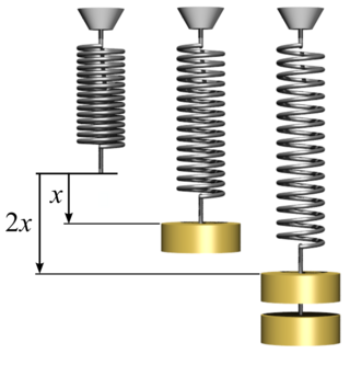
In the tension-compression problem, the following equation shows the relationship between displacement u and force P:

$${\displaystyle {\frac {EA}{L}}u=P}$$

where L is length, A is the area of a cross-section, and E is Young's modulus.

If the Young's modulus and force are uncertain, then

$${\displaystyle E\in [{\underline {E}},{\overline {E}}],P\in [{\underline {P}},{\overline {P}}]}$$

To find upper and lower bounds of the displacement u, calculate the following partial derivatives:

$${\displaystyle {\frac {\partial u}{\partial E}}={\frac {-PL}{E^{2}A}}<0}$$

$${\displaystyle {\frac {\partial u}{\partial P}}={\frac {L}{EA}}>0}$$

Calculate extreme values of the displacement as follows:

$${\displaystyle {\underline {u}}=u({\overline {E}},{\underline {P}})={\frac {{\underline {P}}L}{{\overline {E}}A}}}$$

$${\displaystyle {\overline {u}}=u({\underline {E}},{\overline {P}})={\frac {{\overline {P}}L}{{\underline {E}}A}}}$$

Calculate strain using following formula:

$${\displaystyle \varepsilon ={\frac {1}{L}}u}$$

Calculate derivative of the strain using derivative from the displacements:

$${\displaystyle {\frac {\partial \varepsilon }{\partial E}}={\frac {1}{L}}{\frac {\partial u}{\partial E}}={\frac {-P}{E^{2}A}}<0}$$

$${\displaystyle {\frac {\partial \varepsilon }{\partial P}}={\frac {1}{L}}{\frac {\partial u}{\partial P}}={\frac {1}{EA}}>0}$$

Calculate extreme values of the displacement as follows:

$${\displaystyle {\underline {\varepsilon }}=\varepsilon ({\overline {E}},{\underline {P}})={\frac {\underline {P}}{{\overline {E}}A}}}$$

$${\displaystyle {\overline {\varepsilon }}=\varepsilon ({\underline {E}},{\overline {P}})={\frac {\overline {P}}{{\underline {E}}A}}}$$

It is also possible to calculate extreme values of strain using the displacements

$${\displaystyle {\frac {\partial \varepsilon }{\partial u}}={\frac {1}{L}}>0}$$

then

$${\displaystyle {\underline {\varepsilon }}=\varepsilon ({\underline {u}})={\frac {\underline {P}}{{\overline {E}}A}}}$$

$${\displaystyle {\overline {\varepsilon }}=\varepsilon ({\overline {u}})={\frac {\overline {P}}{{\underline {E}}A}}}$$

The same methodology can be applied to the stress

$${\displaystyle \sigma =E\varepsilon }$$

then

$${\displaystyle {\frac {\partial \sigma }{\partial E}}=\varepsilon +E{\frac {\partial \varepsilon }{\partial E}}=\varepsilon +E{\frac {1}{L}}{\frac {\partial u}{\partial E}}={\frac {P}{EA}}-{\frac {P}{EA}}=0}$$

$${\displaystyle {\frac {\partial \sigma }{\partial P}}=E{\frac {\partial \varepsilon }{\partial P}}=E{\frac {1}{L}}{\frac {\partial u}{\partial P}}={\frac {1}{A}}>0}$$

and

$${\displaystyle {\underline {\sigma }}=\sigma ({\underline {P}})={\frac {\underline {P}}{A}}}$$

$${\displaystyle {\overline {\sigma }}=\sigma ({\overline {P}})={\frac {\overline {P}}{A}}}$$

If we treat stress as a function of strain then

$${\displaystyle {\frac {\partial \sigma }{\partial \varepsilon }}={\frac {\partial }{\partial \varepsilon }}(E\varepsilon )=E>0}$$

then

$${\displaystyle {\underline {\sigma }}=\sigma ({\underline {\varepsilon }})=E{\underline {\varepsilon }}={\frac {\underline {P}}{A}}}$$

$${\displaystyle {\overline {\sigma }}=\sigma ({\overline {\varepsilon }})=E{\overline {\varepsilon }}={\frac {\overline {P}}{A}}}$$

Structure is safe if stress ${\displaystyle \sigma }$ is smaller than a given value ${\displaystyle \sigma _{0}}$ i.e.,

$${\displaystyle \sigma <\sigma _{0}}$$

this condition is true if

$${\displaystyle {\overline {\sigma }}<\sigma _{0}}$$

After calculation we know that this relation is satisfied if

$${\displaystyle {\frac {\overline {P}}{A}}<\sigma _{0}}$$

The example is very simple but it shows the applications of the interval parameters in mechanics. Interval FEM use very similar methodology in multidimensional cases [Pownuk 2004].

However, in the multidimensional cases relation between the uncertain parameters and the solution is not always monotone. In those cases, more complicated optimization methods have to be applied. ^[1]

Multidimensional example

In the case of tension-compression problem the equilibrium equation has the following form

$${\displaystyle {\frac {d}{dx}}\left(EA{\frac {du}{dx}}\right)+n=0}$$

where u is displacement, E is Young's modulus, A is an area of cross-section, and n is a distributed load. In order to get unique solution it is necessary to add appropriate boundary conditions e.g.

$${\displaystyle u(0)=0}$$

$${\displaystyle \left.{\frac {du}{dx}}\right|_{x=0}EA=P}$$

If Young's modulus E and n are uncertain then the interval solution can be defined in the following way

$${\displaystyle {\mathbf {u} }(x)=\left\{u(x):{\frac {d}{dx}}\left(EA{\frac {du}{dx}}\right)+n=0,u(0)=0,{\frac {du(0)}{dx}}EA=P,E\in [{\underline {E}},{\overline {E}}],P\in [{\underline {P}},{\overline {P}}]\right\}}$$

For each FEM element it is possible to multiply the equation by the test function v

$${\displaystyle \int _{0}^{L^{e}}\left({\frac {d}{dx}}\left(EA{\frac {du}{dx}}\right)+n\right)v=0}$$

where ${\displaystyle x\in [0,L^{(e)}].}$

After integration by parts we will get the equation in the weak form

$${\displaystyle \int _{0}^{L^{(e)}}EA{\frac {du}{dx}}{\frac {dv}{dx}}dx=\int _{0}^{L^{(e)}}nv\,dx}$$

where ${\displaystyle x\in [0,L^{(e)}].}$

Let's introduce a set of grid points ${\displaystyle x_{0},x_{1},\dots ,x_{Ne}}$, where ${\displaystyle Ne}$ is a number of elements, and linear shape functions for each FEM element

$${\displaystyle N_{1}^{(e)}(x)=1-{\frac {1-x_{0}^{(e)}}{x_{1}^{(e)}-x_{0}^{(e)}}},\ \ N_{2}^{(e)}(x)={\frac {1-x_{0}^{(e)}}{x_{1}^{(e)}-x_{0}^{(e)}}}.}$$

where ${\displaystyle x\in [x_{0}^{(e)},x_{1}^{(e)}].}$

${\displaystyle x_{1}^{(e)}}$ left endpoint of the element, ${\displaystyle x_{1}^{(e)}}$ left endpoint of the element number "e". Approximate solution in the "e"-th element is a linear combination of the shape functions

$${\displaystyle u_{h}^{(e)}(x)=u_{1}^{e}N_{1}^{(e)}(x)+u_{2}^{e}N_{2}^{(e)}(x),\ \ v_{h}^{(e)}(x)=u_{1}^{e}N_{1}^{(e)}(x)+u_{2}^{e}N_{2}^{(e)}(x)}$$

After substitution to the weak form of the equation we will get the following system of equations

$${\displaystyle {\begin{bmatrix}{\frac {E^{(e)}A^{(e)}}{L^{(e)}}}&-{\frac {E^{(e)}A^{(e)}}{L^{(e)}}}\\-{\frac {E^{(e)}A^{(e)}}{L^{(e)}}}&{\frac {E^{(e)}A^{(e)}}{L^{(e)}}}\\\end{bmatrix}}{\begin{bmatrix}u_{1}^{(e)}\\u_{2}^{(e)}\end{bmatrix}}={\begin{bmatrix}\int _{0}^{L^{(e)}}nN_{1}^{(e)}(x)dx\\\int _{0}^{L^{(e)}}nN_{2}^{(e)}(x)dx\end{bmatrix}}}$$

or in the matrix form

$${\displaystyle K^{(e)}u^{(e)}=Q^{(e)}}$$

In order to assemble the global stiffness matrix it is necessary to consider an equilibrium equations in each node. After that the equation has the following matrix form

$${\displaystyle Ku=Q}$$

where

$${\displaystyle K={\begin{bmatrix}K_{11}^{(1)}&K_{12}^{(1)}&0&\cdots &0\\K_{21}^{(1)}&K_{22}^{(1)}+K_{11}^{(2)}&K_{12}^{(2)}&\cdots &0\\0&K_{21}^{(2)}&K_{22}^{(2)}+K_{11}^{(3)}&\cdots &0\\\vdots &\vdots &\ddots &\ddots &\vdots \\0&0&\cdots &K_{22}^{(Ne-1)}+K_{11}^{(Ne)}&K_{11}^{(Ne)}\\0&0&\cdots &K_{21}^{(Ne)}&K_{22}^{(Ne)}\end{bmatrix}}}$$

is the global stiffness matrix,

$${\displaystyle u={\begin{bmatrix}u_{0}\\u_{1}\\\vdots \\u_{Ne}\\\end{bmatrix}}}$$

is the solution vector,

$${\displaystyle Q={\begin{bmatrix}Q_{0}\\Q_{1}\\\vdots \\Q_{Ne}\\\end{bmatrix}}}$$

is the right hand side.

In the case of tension-compression problem

$${\displaystyle K={\begin{bmatrix}{\frac {E^{(1)}A^{(1)}}{L^{(1)}}}&-{\frac {E^{(1)}A^{(1)}}{L^{(1)}}}&0&\cdots &0\\-{\frac {E^{(1)}A^{(1)}}{L^{(1)}}}&{\frac {E^{(1)}A^{(1)}}{L^{(1)}}}+{\frac {E^{(2)}A^{(2)}}{L^{(2)}}}&-{\frac {E^{(2)}A^{(2)}}{L^{(2)}}}&\cdots &0\\0&-{\frac {E^{(2)}A^{(2)}}{L^{(2)}}}&{\frac {E^{(2)}A^{(2)}}{L^{(2)}}}+{\frac {E^{(3)}A^{(3)}}{L^{(3)}}}&\cdots &0\\\vdots &\vdots &\ddots &\ddots &\vdots \\0&0&\cdots &{\frac {E^{(Ne-1)}A^{(Ne-1)}}{L^{(Ne-1)}}}+{\frac {E^{(Ne)}A^{(Ne)}}{L^{(Ne)}}}&-{\frac {E^{(Ne)}A^{(Ne)}}{L^{(Ne)}}}\\0&0&\cdots &-{\frac {E^{(Ne)}A^{(Ne)}}{L^{(Ne)}}}&{\frac {E^{(Ne)}A^{(Ne)}}{L^{(Ne)}}}\end{bmatrix}}}$$

If we neglect the distributed load n

$${\displaystyle Q={\begin{bmatrix}R\\0\\\vdots \\0\\P\\\end{bmatrix}}}$$

After taking into account the boundary conditions the stiffness matrix has the following form

$${\displaystyle K={\begin{bmatrix}1&0&0&\cdots &0\\0&{\frac {E^{(1)}A^{(1)}}{L^{(1)}}}+{\frac {E^{(2)}A^{(2)}}{L^{(2)}}}&-{\frac {E^{(2)}A^{(2)}}{L^{(2)}}}&\cdots &0\\0&-{\frac {E^{(2)}A^{(2)}}{L^{(2)}}}&{\frac {E^{(2)}A^{(2)}}{L^{(2)}}}+{\frac {E^{(3)}A^{(3)}}{L^{(3)}}}&\cdots &0\\\vdots &\vdots &\ddots &\ddots &\vdots \\0&0&\cdots &{\frac {E^{(e-1)}A^{(e-1)}}{L^{(e-1)}}}+{\frac {E^{(e)}A^{(e)}}{L^{(e)}}}&-{\frac {E^{(e)}A^{(e)}}{L^{(e)}}}\\0&0&\cdots &-{\frac {E^{(e)}A^{(e)}}{L^{(e)}}}&{\frac {E^{(e)}A^{(e)}}{L^{(e)}}}\end{bmatrix}}=K(E,A)=K{\left(E^{(1)},\dots ,E^{(Ne)},A^{(1)},\dots ,A^{(Ne)}\right)}}$$

Right-hand side has the following form

$${\displaystyle Q={\begin{bmatrix}0\\0\\\vdots \\0\\P\\\end{bmatrix}}=Q(P)}$$

Let's assume that Young's modulus E, area of cross-section A and the load P are uncertain and belong to some intervals

$${\displaystyle E^{(e)}\in [{\underline {E}}^{(e)},{\overline {E}}^{(e)}]}$$

$${\displaystyle A^{(e)}\in [{\underline {A}}^{(e)},{\overline {A}}^{(e)}]}$$

$${\displaystyle P\in [{\underline {P}},{\overline {P}}]}$$

The interval solution can be defined calculating the following way

$${\displaystyle \mathbf {u} =\lozenge \left\{u:K(E,A)u=Q(P),E^{(e)}\in [{\underline {E}}^{(e)},{\overline {E}}^{(e)}],A^{(e)}\in [{\underline {A}}^{(e)},{\overline {A}}^{(e)}],P\in [{\underline {P}},{\overline {P}}]\right\}}$$

Calculation of the interval vector ${\displaystyle {\mathbf {u} }}$ is in general NP-hard, however in specific cases it is possible to calculate the solution which can be used in many engineering applications.

The results of the calculations are the interval displacements

$${\displaystyle u_{i}\in [{\underline {u}}_{i},{\overline {u}}_{i}]}$$

Let's assume that the displacements in the column have to be smaller than some given value (due to safety).

$${\displaystyle u_{i}<u_{i}^{\max }}$$

The uncertain system is safe if the interval solution satisfy all safety conditions.

In this particular case

$${\displaystyle u_{i}<u_{i}^{\max },\ \ \ u_{i}\in [{\underline {u}}_{i},{\overline {u}}_{i}]}$$

or simple

$${\displaystyle {\overline {u}}_{i}<u_{i}^{\max }}$$

In postprocessing it is possible to calculate the interval stress, the interval strain and the interval limit state functions and use these values in the design process.

The interval finite element method can be applied to the solution of problems in which there is not enough information to create reliable probabilistic characteristic of the structures (Elishakoff 2000). Interval finite element method can be also applied in the theory of imprecise probability.

Endpoints combination method

It is possible to solve the equation ${\displaystyle K(p)u(p)=Q(p)}$ for all possible combinations of endpoints of the interval ${\displaystyle {\hat {p}}}$.
The list of all vertices of the interval ${\displaystyle {\hat {p}}}$ can be written as ${\displaystyle L=\{p_{1}^{*},...,p_{n}^{*}\}}$.
Upper and lower bound of the solution can be calculated in the following way

$${\displaystyle {\underline {u}}_{i}=\min\{u_{i}(p_{k}^{*}):K(p_{k}^{*})u(p_{k}^{*})=Q(p_{k}^{*}),p_{k}^{*}\in L\}}$$

$${\displaystyle {\overline {u}}_{i}=\max\{u_{i}(p_{k}^{*}):K(p_{k}^{*})u(p_{k}^{*})=Q(p_{k}^{*}),p_{k}^{*}\in L\}}$$

Endpoints combination method gives solution which is usually exact; unfortunately the method has exponential computational complexity and cannot be applied to the problems with many interval parameters. ^[3]

Taylor expansion method

The function ${\displaystyle u=u(p)}$ can be expanded by using Taylor series. In the simplest case the Taylor series use only linear approximation

$${\displaystyle u_{i}(p)\approx u_{i}(p_{0})+\sum _{j}{\frac {\partial u(p_{0})}{\partial p_{j}}}\Delta p_{j}}$$

Upper and lower bound of the solution can be calculated by using the following formula

$${\displaystyle {\underline {u}}_{i}\approx u_{i}(p_{0})-\left|\sum _{j}{\frac {\partial u(p_{0})}{\partial p_{j}}}\right|\Delta p_{j}}$$

$${\displaystyle {\overline {u}}_{i}\approx u_{i}(p_{0})+\left|\sum _{j}{\frac {\partial u(p_{0})}{\partial p_{j}}}\right|\Delta p_{j}}$$

The method is very efficient however it is not very accurate.
In order to improve accuracy it is possible to apply higher order Taylor expansion [Pownuk 2004].
This approach can be also applied in the interval finite difference method and the interval boundary element method.

Gradient method

If the sign of the derivatives ${\displaystyle {\frac {\partial u_{i}}{\partial p_{j}}}}$ is constant then the functions ${\displaystyle u_{i}=u_{i}(p)}$ is monotone and the exact solution can be calculated very fast.

if ${\displaystyle {\frac {\partial u_{i}}{\partial p_{j}}}\geq 0}$ then ${\displaystyle p_{i}^{\min }={\underline {p}}_{i},\ p_{i}^{\max }={\overline {p}}_{i}}$

if ${\displaystyle {\frac {\partial u_{i}}{\partial p_{j}}}<0}$ then ${\displaystyle p_{i}^{\min }={\overline {p}}_{i},\ p_{i}^{\max }={\underline {p}}_{i}}$

Extreme values of the solution can be calculated in the following way

$${\displaystyle {\underline {u}}_{i}=u_{i}(p^{\min }),\ {\overline {u}}_{i}=u_{i}(p^{\max })}$$

In many structural engineering applications the method gives exact solution.
If the solution is not monotone the solution is usually reasonable. In order to improve accuracy of the method it is possible to apply monotonicity tests and higher order sensitivity analysis. The method can be applied to the solution of linear and nonlinear problems of computational mechanics [Pownuk 2004]. Applications of sensitivity analysis method to the solution of civil engineering problems can be found in the following paper [M.V. Rama Rao, A. Pownuk and I. Skalna 2008].
This approach can be also applied in the interval finite difference method and the interval boundary element method.

Element by element method

Muhanna and Mullen applied element by element formulation to the solution of finite element equation with the interval parameters. ^[4] Using that method it is possible to get the solution with guaranteed accuracy in the case of truss and frame structures.

Perturbation methods

The solution ${\displaystyle u=u(p)}$ stiffness matrix ${\displaystyle K=K(p)}$ and the load vector ${\displaystyle Q=Q(p)}$ can be expanded by using perturbation theory. Perturbation theory lead to the approximate value of the interval solution. ^[5] The method is very efficient and can be applied to large problems of computational mechanics.

Response surface method

It is possible to approximate the solution ${\displaystyle u=u(p)}$ by using response surface. Then it is possible to use the response surface to the get the interval solution. ^[6] Using response surface method it is possible to solve very complex problem of computational mechanics. ^[7]

Pure interval methods

Several authors tried to apply pure interval methods to the solution of finite element problems with the interval parameters. In some cases it is possible to get very interesting results e.g. [Popova, Iankov, Bonev 2008]. However, in general the method generates very overestimated results. ^[8]

Parametric interval systems

Popova ^[9] and Skalna ^[10] introduced the methods for the solution of the system of linear equations in which the coefficients are linear combinations of interval parameters. In this case it is possible to get very accurate solution of the interval equations with guaranteed accuracy.

See also

• Interval boundary element method
• Interval (mathematics)
• Interval arithmetic
• Imprecise probability
• Multivalued function
• Differential inclusion
• Observational error
• Random compact set
• Reliability (statistics)
• Confidence interval
• Best, worst and average case
• Probabilistic design
• Propagation of uncertainty
• Experimental uncertainty analysis
• Sensitivity analysis
• Perturbation theory
• Continuum mechanics
• Solid mechanics
• Truss
• Space frame
• Linear elasticity
• Strength of materials

References

1. "Interval equations". Archived from the original on 2011-10-05. Retrieved 2008-10-12.
2. E. Popova, Parametric Solution Set of Interval Linear System Archived 2010-01-27 at the Wayback Machine
3. A. Neumaier, Interval methods for systems of equations, Cambridge University Press, New York, 1990
4. R.L. Muhanna, R.L. Mullen, Uncertainty in Mechanics Problems - Interval - Based Approach. Journal of Engineering Mechanics, Vol.127, No.6, 2001, 557-556
5. Z. Qiu and I. Elishakoff, Antioptimization of structures with large uncertain but non-random parameters via interval analysis Computer Methods in Applied Mechanics and Engineering, Volume 152, Issues 3-4, 24 January 1998, Pages 361-372
6. U.O. Akpan, T.S. Koko, I.R. Orisamolu, B.K. Gallant, Practical fuzzy finite element analysis of structures, Finite Elements in Analysis and Design, 38, pp. 93–111, 2000.
7. M. Beer, Evaluation of Inconsistent Engineering data, The Third workshop on Reliable Engineering Computing (REC08) Georgia Institute of Technology, February 20–22, 2008, Savannah, Georgia, USA.
8. Kulpa Z., Pownuk A., Skalna I., Analysis of linear mechanical structures with uncertainties by means of interval methods. Computer Assisted Mechanics and Engineering Sciences, vol. 5, 1998, pp. 443–477
9. E. Popova, On the Solution of Parametrised Linear Systems. W. Kraemer, J. Wolff von Gudenberg (Eds.): Scientific Computing,Validated Numerics, Interval Methods. Kluwer Acad. Publishers, 2001, pp. 127–138.
10. I. Skalna, A Method for Outer Interval Solution of Systems of Linear Equations Depending Linearly on Interval Parameters, Reliable Computing, Volume 12, Number 2, April, 2006, pp. 107–120

• Dempster, A. P. (1967). "Upper and lower probabilities induced by a multivalued mapping". The Annals of Mathematical Statistics 38 (2): 325–339. . Retrieved 2009-09-23
• Analyzing Uncertainty in Civil Engineering, by W. Fellin, H. Lessmann, M. Oberguggenberger, and R. Vieider (eds.), Springer-Verlag, Berlin, 2005
• I. Elishakoff, Possible limitations of probabilistic methods in engineering. Applied Mechanics Reviews, Vol.53, No.2, pp. 19–25, 2000.
• Hlavácek, I., Chleboun, J., Babuška, I.: Uncertain Input Data Problems and the Worst Scenario Method. Elsevier, Amsterdam (2004)
• Köylüoglu, U., Isaac Elishakoff; A comparison of stochastic and interval finite elements applied to shear frames with uncertain stiffness properties, Computers & Structures Volume: 67, Issue: 1–3, April 1, 1998, pp. 91–98
• D. Moens and D. Vandepitte, Interval sensitivity theory and its application to frequency response envelope analysis of uncertain structures. Computer Methods in Applied Mechanics and Engineering Vol. 196, No. 21-24,1 April 2007, pp. 2486–2496.
• Möller, B., Beer, M., Fuzzy Randomness - Uncertainty in Civil Engineering and Computational Mechanics, Springer, Berlin, 2004.
• E. Popova, R. Iankov, Z. Bonev: Bounding the Response of Mechanical Structures with Uncertainties in all the Parameters. In R.L.Muhannah, R.L.Mullen (Eds): Proceedings of the NSF Workshop on Reliable Engineering Computing (REC), Svannah, Georgia USA, Feb. 22–24, 2006, 245-265
• A. Pownuk, Numerical solutions of fuzzy partial differential equation and its application in computational mechanics, Fuzzy Partial Differential Equations and Relational Equations: Reservoir Characterization and Modeling (M. Nikravesh, L. Zadeh and V. Korotkikh, eds.), Studies in Fuzziness and Soft Computing, Physica-Verlag, 2004, pp. 308–347
• A. Pownuk, Efficient Method of Solution of Large Scale Engineering Problems with Interval Parameters Based on Sensitivity Analysis, Proceeding of NSF workshop on Reliable Engineering Computing, September 15–17, 2004, Savannah, Georgia, USA, pp. 305–316
• M.V. Rama Rao, A. Pownuk and I. Skalna, Stress Analysis of a Singly Reinforced Concrete Beam with Uncertain Structural Parameters, NSF workshop on Reliable Engineering Computing, February 20–22, 2008, Savannah, Georgia, USA, pp. 459–478
• Bernardini, Alberto, Tonon, Fulvio, Bounding Uncertainty in Civil Engineering, Springer 2010
• Ben-Haim Y., Elishakoff I., 1990, Convex Models of Uncertainty in Applied Mechanics. Elsevier Science Publishers, New York
• Valliappan S., Pham T.D., 1993, Fuzzy Finite Element Analysis of A Foundation on Elastic Soil Medium. International Journal for Numerical and Analytical Methods in Geomechanics, Vol.17, pp. 771–789
• Elishakoff I., Li Y.W., Starnes J.H., 1994, A deterministic method to predict the effect of unknown-but-bounded elastic moduli on the buckling of composite structures. Computer methods in applied mechanics and engineering, Vol.111, pp. 155–167
• Valliappan S. Pham T.D., 1995, Elasto-Plastic Finite Element Analysis with Fuzzy Parameters. International Journal for Numerical Methods in Engineering, 38, pp. 531–548
• Rao S.S., Sawyer J.P., 1995, Fuzzy Finite Element Approach for the Analysis of Imprecisly Defined Systems. AIAA Journal, Vol.33, No.12, pp. 2364–2370
• Köylüoglu H.U., Cakmak A., Nielsen S.R.K., 1995, Interval mapping in structural mechanics. In: Spanos, ed. Computational Stochastic Mechanics. 125–133. Balkema, Rotterdam
• Muhanna, R. L. and R. L. Mullen (1995). "Development of Interval Based Methods for Fuzziness in Continuum Mechanics" in Proceedings of the 3rd International Symposium on Uncertainty Modeling and Analysis and Annual Conference of the North American Fuzzy Information Processing Society (ISUMA–NAFIPS'95),IEEE, 705–710

External links

• Reliable Engineering Computing, Georgia Institute of Technology, Savannah, USA
• Interval Computations
• Reliable Computing (Journal)
• Interval equations (collections of references)
• Interval finite element web applications
• E. Popova, Parametric Solution Set of Interval Linear System
• The Society for Imprecise Probability: Theories and Applications