Eddy (fluid dynamics)

A vortex street around a cylinder. This can occur around cylinders and spheres, for any fluid, cylinder size and fluid speed, provided that the flow has a Reynolds number in the range ~40 to ~1000.

In fluid dynamics, an eddy is the swirling of a fluid and the reverse current created when the fluid is in a turbulent flow regime. ^[2] The moving fluid creates a space devoid of downstream-flowing fluid on the downstream side of the object. Fluid behind the obstacle flows into the void creating a swirl of fluid on each edge of the obstacle, followed by a short reverse flow of fluid behind the obstacle flowing upstream, toward the back of the obstacle. This phenomenon is naturally observed behind large emergent rocks in swift-flowing rivers.

An eddy is a movement of fluid that deviates from the general flow of the fluid. An example for an eddy is a vortex which produces such deviation. However, there are other types of eddies that are not simple vortices. For example, a Rossby wave is an eddy ^[3] which is an undulation that is a deviation from mean flow, but does not have the local closed streamlines of a vortex.

Swirl and eddies in engineering

The propensity of a fluid to swirl is used to promote good fuel/air mixing in internal combustion engines.

In fluid mechanics and transport phenomena, an eddy is not a property of the fluid, but a violent swirling motion caused by the position and direction of turbulent flow. ^[4]

A diagram showing the velocity distribution of a fluid moving through a circular pipe, for laminar flow (left), time-averaged (center), and turbulent flow, instantaneous depiction (right)

Reynolds number and turbulence

Reynolds Experiment (1883). Osborne Reynolds standing beside his apparatus.

In 1883, scientist Osborne Reynolds conducted a fluid dynamics experiment involving water and dye, where he adjusted the velocities of the fluids and observed the transition from laminar to turbulent flow, characterized by the formation of eddies and vortices. ^[5] Turbulent flow is defined as the flow in which the system's inertial forces are dominant over the viscous forces. This phenomenon is described by Reynolds number, a unit-less number used to determine when turbulent flow will occur. Conceptually, the Reynolds number is the ratio between inertial forces and viscous forces. ^[6]

Schlieren photograph showing the thermal convection plume rising from an ordinary candle in still air. The plume is initially laminar, but transition to turbulence occurs in the upper third of the image. The image was made by Gary Settles using a one-meter-diameter schlieren mirror.

The general form for the Reynolds number flowing through a tube of radius r (or diameter d):

${\displaystyle \mathrm {Re} ={\frac {2v\rho r}{\mu }}={\frac {\rho vd}{\mu }}}$

where v is the velocity of the fluid, ρ is its density, r is the radius of the tube, and μ is the dynamic viscosity of the fluid. A turbulent flow in a fluid is defined by the critical Reynolds number, for a closed pipe this works out to approximately

${\displaystyle \mathrm {Re} _{\text{c}}\approx 2000.}$

In terms of the critical Reynolds number, the critical velocity is represented as

${\displaystyle v_{\text{c}}={\frac {\mathrm {Re} _{\text{c}}\mu }{\rho d}}.}$

Research and development

Computational fluid dynamics

These are turbulence models in which the Reynolds stresses, as obtained from a Reynolds averaging of the Navier–Stokes equations, are modelled by a linear constitutive relationship with the mean flow straining field, as:

${\displaystyle -\rho \langle u_{i}u_{j}\rangle =2\mu _{t}S_{i,j}-{\tfrac {2}{3}}\rho \kappa \delta _{i,j}}$

where

• ${\displaystyle \mu _{t}}$ is the coefficient termed turbulence "viscosity" (also called the eddy viscosity)
• ${\displaystyle \kappa ={\tfrac {1}{2}}{\bigl (}\langle u_{1}u_{1}\rangle +\langle u_{2}u_{2}\rangle +\langle u_{3}u_{3}\rangle {\bigr )}}$ is the mean turbulent kinetic energy
• ${\displaystyle S_{i,j}}$ is the mean strain rate

Note that that inclusion of ${\displaystyle {\tfrac {2}{3}}\rho \kappa \delta _{i,j}}$ in the linear constitutive relation is required by tensorial algebra purposes when solving for two-equation turbulence models (or any other turbulence model that solves a transport equation for ${\displaystyle \kappa }$ . ^[7]

Hemodynamics

Hemodynamics is the study of blood flow in the circulatory system. Blood flow in straight sections of the arterial tree are typically laminar (high, directed wall stress), but branches and curvatures in the system cause turbulent flow. ^[2] Turbulent flow in the arterial tree can cause a number of concerning effects, including atherosclerotic lesions, postsurgical neointimal hyperplasia, in-stent restenosis, vein bypass graft failure, transplant vasculopathy, and aortic valve calcification.

Industrial processes

Lift and drag properties of golf balls are customized by the manipulation of dimples along the surface of the ball, allowing for the golf ball to travel further and faster in the air. ^{[8] [9]} The data from turbulent-flow phenomena has been used to model different transitions in fluid flow regimes, which are used to thoroughly mix fluids and increase reaction rates within industrial processes. ^[10]

Fluid currents and pollution control

Oceanic and atmospheric currents transfer particles, debris, and organisms all across the globe. While the transport of organisms, such as phytoplankton, are essential for the preservation of ecosystems, oil and other pollutants are also mixed in the current flow and can carry pollution far from its origin. ^{[11] [12]} Eddy formations circulate trash and other pollutants into concentrated areas which researchers are tracking to improve clean-up and pollution prevention. The distribution and motion of plastics caused by eddy formations in natural water bodies can be predicted using Lagrangian transport models. ^[13] Mesoscale ocean eddies play crucial roles in transferring heat poleward, as well as maintaining heat gradients at different depths. ^[14]

Environmental flows

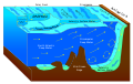
Modeling eddy development, as it relates to turbulence and fate transport phenomena, is vital in grasping an understanding of environmental systems. By understanding the transport of both particulate and dissolved solids in environmental flows, scientists and engineers will be able to efficiently formulate remediation strategies for pollution events. Eddy formations play a vital role in the fate and transport of solutes and particles in environmental flows such as in rivers, lakes, oceans, and the atmosphere. Upwelling in stratified coastal estuaries warrant the formation of dynamic eddies which distribute nutrients out from beneath the boundary layer to form plumes. ^[15] Shallow waters, such as those along the coast, play a complex role in the transport of nutrients and pollutants due to the proximity of the upper-boundary driven by the wind and the lower-boundary near the bottom of the water body. ^[16]

Mesoscale ocean eddies

Downwind of obstacles, in this case, the Madeira and the Canary Islands off the west African coast, eddies create turbulent patterns called vortex streets.

Eddies are common in the ocean, and range in diameter from centimeters to hundreds of kilometers. The smallest scale eddies may last for a matter of seconds, while the larger features may persist for months to years.

Eddies that are between about 10 and 500 km (6 and 300 miles) in diameter and persist for periods of days to months are known in oceanography as mesoscale eddies. ^[17]

Mesoscale eddies can be split into two categories: static eddies, caused by flow around an obstacle (see animation)^{[ clarification needed ]}, and transient eddies, caused by baroclinic instability.

When the ocean contains a sea surface height gradient this creates a jet or current, such as the Antarctic Circumpolar Current. This current as part of a baroclinically unstable system meanders and creates eddies (in much the same way as a meandering river forms an oxbow lake). These types of mesoscale eddies have been observed in many major ocean currents, including the Gulf Stream, the Agulhas Current, the Kuroshio Current, and the Antarctic Circumpolar Current, amongst others.

Mesoscale ocean eddies are characterized by currents that flow in a roughly circular motion around the center of the eddy. The sense of rotation of these currents may either be cyclonic or anticyclonic (such as Haida Eddies). Oceanic eddies are also usually made of water masses that are different from those outside the eddy. That is, the water within an eddy usually has different temperature and salinity characteristics to the water outside the eddy. There is a direct link between the water mass properties of an eddy and its rotation. Warm eddies rotate anti-cyclonically, while cold eddies rotate cyclonically.

Because eddies may have a vigorous circulation associated with them, they are of concern to naval and commercial operations at sea. Further, because eddies transport anomalously warm or cold water as they move, they have an important influence on heat transport in certain parts of the ocean. ^[18]

Influences on apex predators

The sub-tropical Northern Atlantic is known to have both cyclonic and anticyclonic eddies that are associated with high surface chlorophyll and low surface chlorophyll, respectively. The presence of chlorophyll and higher levels of chlorophyll allows this region to support higher biomass of phytoplankton, as well as, supported by areas of increased vertical nutrient fluxes and transportation of biological communities. This area of the Atlantic is also thought to be an ocean desert, which creates an interesting paradox due to it hosting a variety of large pelagic fish populations and apex predators ^{[19] [20] [21]}

These mesoscale eddies have shown to be beneficial in further creating ecosystem-based management for food web models to better understand the utilization of these eddies by both the apex predators and their prey. Gaube et al. (2018), used “Smart” Position or Temperature Transmitting tags (SPOT) and Pop-Up Satellite Archival Transmitting tags (PSAT) to track the movement and diving behavior of two female white sharks (Carcharodon carcharias) within the eddies. The eddies were defined using sea surface height (SSH) and contours using the horizontal speed-based radius scale. This study found that the white sharks dove in both cyclones but favored the anticyclone which had three times more dives as the cyclonic eddies. Additionally, in the Gulf Stream eddies, the anticyclonic eddies were 57% more common and had more dives and deeper dives than the open ocean eddies and Gulf Stream cyclonic eddies. ^[21]

Within these anticyclonic eddies, the isotherm was displaced 50 meters downward allowing for the warmer water to penetrate deeper in the water column. This warmer water displacement may allow for the white sharks to make longer dives without the added energetic cost from thermal regulation in the cooler cyclones. Even though these anticyclonic eddies resulted in lower levels of chlorophyll in comparison to the cyclonic eddies, the warmer waters at deeper depths may allow for a deeper mixed layer and higher concentration of diatoms which in turn result in higher rates of primary productivity. ^{[21] [22]} Furthermore, the prey populations could be distributed more within these eddies attracting these larger female sharks to forage in this mesopelagic zone. This diving pattern may follow a diel vertical migration but without more evidence on the biomass of their prey within this zone, these conclusions cannot be made only using this circumstantial evidence. ^[21]

The biomass in the mesopelagic zone is still understudied leading to the biomass of fish within this layer to potentially be underestimated. A more accurate measurement on this biomass may serve to benefit the commercial fishing industry providing them with additional fishing grounds within this region. Moreover, further understanding this region in the open ocean and how the removal of fish in this region may impact this pelagic food web is crucial for the fish populations and apex predators that may rely on this food source in addition to making better ecosystem-based management plans. ^[21]

See also

• Vortex
• Eddy pumping - component of vertical motion in eddies relevant for biology and biogeochemistry
• Eddy diffusion
• Haida Eddies
• Irminger Rings
• Reynolds number - a dimensionless constant used to predict the onset of turbulent flow
• Reynolds experiment
• Kármán vortex street
• Whirlpool
• Whirlwind
• River eddies in whitewater
• Wake turbulence
• Computational fluid dynamics
• Laminar flow
• Hemodynamics
• Modons, or dipole eddy pairs.

References

1. Tansley, Claire E.; Marshall, David P. (2001). "Flow past a Cylinder on a Plane, with Application to Gulf Stream Separation and the Antarctic Circumpolar Current" (PDF). Journal of Physical Oceanography. 31 (11): 3274–3283. Bibcode:2001JPO....31.3274T. doi:10.1175/1520-0485(2001)031<3274:FPACOA>2.0.CO;2. Archived from the original (PDF) on 2011-04-01.
2. Chiu, Jeng-Jiann; Chien, Shu (2011-01-01). "Effects of Disturbed Flow on Vascular Endothelium: Pathophysiological Basis and Clinical Perspectives". Physiological Reviews. 91 (1): 327–387. doi:10.1152/physrev.00047.2009. ISSN   0031-9333. PMC   3844671 . PMID   21248169.
3. Encyclopedia Britannica eddy (fluid-mechanics)
4. Lightfoot, R. Byron Bird; Warren E. Stewart; Edwin N. (2002). Transport phenomena (2. ed.). New York, NY [u.a.]: Wiley. ISBN   0-471-41077-2.
5. Kambe, Tsutomu (2007). Elementary Fluid Mechanics . World Scientific Publishing Co. Pte. Ltd. pp.  240. ISBN   978-981-256-416-0.
6. "Pressure". hyperphysics.phy-astr.gsu.edu. Retrieved 2017-02-12.
7. "Linear eddy viscosity models -- CFD-Wiki, the free CFD reference". www.cfd-online.com. Retrieved 2017-02-12.
8. Arnold, Douglas. "The Flight of a Golf Ball" (PDF).
9. "Why are Golf Balls Dimpled?". math.ucr.edu. Retrieved 2017-02-12.
10. Dimotakis, Paul. "The Mixing Transition in Turbulent Flows" (PDF). California Institute of Technology Information Tech Services.
11. "Ocean currents push phytoplankton, and pollution, around the globe faster than thought". Science Daily . 16 April 2016. Retrieved 2017-02-12.
12. "Ocean Pollution". National Oceanic and Atmospheric Administration.
13. Daily, Juliette; Hoffman, Matthew J. (2020-05-01). "Modeling the three-dimensional transport and distribution of multiple microplastic polymer types in Lake Erie". Marine Pollution Bulletin. 154: 111024. doi: 10.1016/j.marpolbul.2020.111024 . ISSN   0025-326X. PMID   32319887.
14. "Ocean Mesoscale Eddies – Geophysical Fluid Dynamics Laboratory". www.gfdl.noaa.gov. Retrieved 2017-02-12.
15. Chen, Zhaoyun; Jiang, Yuwu; Wang, Jia; Gong, Wenping (2019-07-23). "Influence of a River Plume on Coastal Upwelling Dynamics: Importance of Stratification". Journal of Physical Oceanography. 49 (9): 2345–2363. Bibcode:2019JPO....49.2345C. doi: 10.1175/JPO-D-18-0215.1 . ISSN   0022-3670.
16. Roman, F.; Stipcich, G.; Armenio, V.; Inghilesi, R.; Corsini, S. (2010-06-01). "Large eddy simulation of mixing in coastal areas". International Journal of Heat and Fluid Flow. Sixth International Symposium on Turbulence and Shear Flow Phenomena. 31 (3): 327–341. doi:10.1016/j.ijheatfluidflow.2010.02.006. ISSN   0142-727X. S2CID   123151803.
17. Tansley, Claire E.; Marshall, David P. (2001). "Flow past a Cylinder on a β Plane, with Application to Gulf Stream Separation and the Antarctic Circumpolar Current". Journal of Physical Oceanography. 31 (11): 3274–3283. Bibcode:2001JPO....31.3274T. doi: 10.1175/1520-0485(2001)031<3274:FPACOA>2.0.CO;2 . ISSN   1520-0485. S2CID   130455873.
18. "Ocean Mesoscale Eddies". Geophysical Fluid Dynamics Laboratory . NOAA . Retrieved 2021-06-10.
19. Chelton, D. B., Gaube, P., Schlax, M. G., Early, J. J., & Samelson, R. M. (2011). The influence of nonlinear mesoscale eddies on near-surface oceanic chlorophyll. Science, 334(6054). https://doi.org/10.1126/science.1208897
20. Gaube, P., McGillicuddy, D. J., Chelton, D. B., Behrenfeld, M. J., & Strutton, P. G. (2014). Regional variations in the influence of mesoscale eddies on near-surface chlorophyll. Journal of Geophysical Research: Oceans, 119(12). https://doi.org/10.1002/2014JC010111
21. Gaube, P., Braun, C. D., Lawson, G. L., McGillicuddy, D. J., Penna, A. della, Skomal, G. B., Fischer, C., & Thorrold, S. R. (2018). Mesoscale eddies influence the movements of mature female white sharks in the Gulf Stream and Sargasso Sea. Scientific Reports, 8(1). https://doi.org/10.1038/S41598-018-25565-8
22. McGillicuddy, D. J., Anderson, L. A., Bates, N. R., Bibby, T., Buesseler, K. O., Carlson, C. A., Davis, C. S., Ewart, C., Falkowski, P. G., Goldthwait, S. A., Hansell, D. A., Jenkins, W. J., Johnson, R., Kosnyrev, V. K., Ledwell, J. R., Li, Q. P., Siegel, D. A., & Steinberg, D. K. (2007). Eddy/Wind interactions stimulate extraordinary mid-ocean plankton blooms. Science, 316(5827). https://doi.org/10.1126/science.1136256