Stokes drift

An expanse of driftwood along the northern coast of Washington state. Stokes drift – besides e.g. Ekman drift and geostrophic currents – is one of the relevant processes in the transport of marine debris.

For a pure wave motion in fluid dynamics, the Stokes drift velocity is the average velocity when following a specific fluid parcel as it travels with the fluid flow. For instance, a particle floating at the free surface of water waves, experiences a net Stokes drift velocity in the direction of wave propagation.

More generally, the Stokes drift velocity is the difference between the average Lagrangian flow velocity of a fluid parcel, and the average Eulerian flow velocity of the fluid at a fixed position. This nonlinear phenomenon is named after George Gabriel Stokes, who derived expressions for this drift in his 1847 study of water waves.

The Stokes drift is the difference in end positions, after a predefined amount of time (usually one wave period), as derived from a description in the Lagrangian and Eulerian coordinates. The end position in the Lagrangian description is obtained by following a specific fluid parcel during the time interval. The corresponding end position in the Eulerian description is obtained by integrating the flow velocity at a fixed position—equal to the initial position in the Lagrangian description—during the same time interval.

The Stokes drift velocity equals the Stokes drift divided by the considered time interval. Often, the Stokes drift velocity is loosely referred to as Stokes drift. Stokes drift may occur in all instances of oscillatory flow which are inhomogeneous in space. For instance in water waves, tides and atmospheric waves.

In the Lagrangian description, fluid parcels may drift far from their initial positions. As a result, the unambiguous definition of an average Lagrangian velocity and Stokes drift velocity, which can be attributed to a certain fixed position, is by no means a trivial task. However, such an unambiguous description is provided by the Generalized Lagrangian Mean (GLM) theory of Andrews and McIntyre in 1978. ^[2]

The Stokes drift is important for the mass transfer of various kinds of material and organisms by oscillatory flows. It plays a crucial role in the generation of Langmuir circulations. ^[3] For nonlinear and periodic water waves, accurate results on the Stokes drift have been computed and tabulated. ^[4]

Mathematical description

Stokes drift in deep water waves, with a wave length of about twice the water depth.

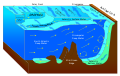
Stokes drift in shallow water waves, with a wave length much longer than the water depth.

The red circles are the present positions of massless particles, moving with the flow velocity. The light-blue line gives the path of these particles, and the light-blue circles the particle position after each wave period. The white dots are fluid particles, also followed in time. In the cases shown here, the mean Eulerian horizontal velocity below the wave trough is zero.
Observe that the wave period, experienced by a fluid particle near the free surface, is different from the wave period at a fixed horizontal position (as indicated by the light-blue circles). This is due to the Doppler shift.

The Lagrangian motion of a fluid parcel with position vector x = ξ(α, t) in the Eulerian coordinates is given by ^[5]

${\displaystyle {\dot {\boldsymbol {\xi }}}={\frac {\partial {\boldsymbol {\xi }}}{\partial t}}=\mathbf {u} {\big (}{\boldsymbol {\xi }}({\boldsymbol {\alpha }},t),t{\big )},}$

where

∂ξ/∂t is the partial derivative of ξ(α, t) with respect to t,

ξ(α, t) is the Lagrangian position vector of a fluid parcel,

u(x, t) is the Eulerian velocity,

x is the position vector in the Eulerian coordinate system,

α is the position vector in the Lagrangian coordinate system,

t is time.

Often, the Lagrangian coordinates α are chosen to coincide with the Eulerian coordinates x at the initial time t = t₀: ^[5]

${\displaystyle {\boldsymbol {\xi }}({\boldsymbol {\alpha }},t_{0})={\boldsymbol {\alpha }}.}$

If the average value of a quantity is denoted by an overbar, then the average Eulerian velocity vector ū_E and average Lagrangian velocity vector ū_L are

${\displaystyle {\begin{aligned}{\bar {\mathbf {u} }}_{\text{E}}&={\overline {\mathbf {u} (\mathbf {x} ,t)}},\\{\bar {\mathbf {u} }}_{\text{L}}&={\overline {{\dot {\boldsymbol {\xi }}}({\boldsymbol {\alpha }},t)}}={\overline {\left({\frac {\partial {\boldsymbol {\xi }}({\boldsymbol {\alpha }},t)}{\partial t}}\right)}}={\overline {{\boldsymbol {u}}{\big (}{\boldsymbol {\xi }}({\boldsymbol {\alpha }},t),t{\big )}}}.\end{aligned}}}$

Different definitions of the average may be used, depending on the subject of study (see ergodic theory):

• time average,
• space average,
• ensemble average,
• phase average.

The Stokes drift velocity ū_S is defined as the difference between the average Eulerian velocity and the average Lagrangian velocity: ^[6]

${\displaystyle {\bar {\mathbf {u} }}_{\text{S}}={\bar {\mathbf {u} }}_{\text{L}}-{\bar {\mathbf {u} }}_{\text{E}}.}$

In many situations, the mapping of average quantities from some Eulerian position x to a corresponding Lagrangian position α forms a problem. Since a fluid parcel with label α traverses along a path of many different Eulerian positions x, it is not possible to assign α to a unique x. A mathematically sound basis for an unambiguous mapping between average Lagrangian and Eulerian quantities is provided by the theory of the generalized Lagrangian mean (GLM) by Andrews and McIntyre (1978).

Example: A one-dimensional compressible flow

For the Eulerian velocity as a monochromatic wave of any nature in a continuous medium: ${\displaystyle u={\hat {u}}\sin(kx-\omega t),}$ one readily obtains by the perturbation theory  – with ${\displaystyle k{\hat {u}}/\omega }$ as a small parameter – for the particle position ${\displaystyle x=\xi (\xi _{0},t)}$:

${\displaystyle {\dot {\xi }}=u(\xi ,t)={\hat {u}}\sin(k\xi -\omega t),}$

${\displaystyle \xi (\xi _{0},t)\approx \xi _{0}+{\frac {\hat {u}}{\omega }}\cos(k\xi _{0}-\omega t)-{\frac {1}{4}}{\frac {k{\hat {u}}^{2}}{\omega ^{2}}}\sin 2(k\xi _{0}-\omega t)+{\frac {1}{2}}{\frac {k{\hat {u}}^{2}}{\omega }}t.}$

Here the last term describes the Stokes drift velocity ${\displaystyle {\tfrac {1}{2}}k{\hat {u}}^{2}/\omega .}$ ^[7]

Example: Deep water waves

Stokes drift under periodic waves in deep water, for a period T = 5 s and a mean water depth of 25 m. Left: instantaneous horizontal flow velocities. Right: average flow velocities. Black solid line: average Eulerian velocity; red dashed line: average Lagrangian velocity, as derived from the Generalized Lagrangian Mean (GLM).

See also: Airy wave theory and Stokes wave

The Stokes drift was formulated for water waves by George Gabriel Stokes in 1847. For simplicity, the case of infinitely deep water is considered, with linear wave propagation of a sinusoidal wave on the free surface of a fluid layer: ^[8]

${\displaystyle \eta =a\cos(kx-\omega t),}$

where

η is the elevation of the free surface in the z direction (meters),

a is the wave amplitude (meters),

k is the wave number: k = 2π/λ (radians per meter),

ω is the angular frequency: ω = 2π/T (radians per second),

x is the horizontal coordinate and the wave propagation direction (meters),

z is the vertical coordinate, with the positive z direction pointing out of the fluid layer (meters),

λ is the wave length (meters),

T is the wave period (seconds).

As derived below, the horizontal component ū_S(z) of the Stokes drift velocity for deep-water waves is approximately: ^[9]

${\displaystyle {\bar {u}}_{\text{S}}\approx \omega ka^{2}{\text{e}}^{2kz}={\frac {4\pi ^{2}a^{2}}{\lambda T}}{\text{e}}^{4\pi z/\lambda }.}$

As can be seen, the Stokes drift velocity ū_S is a nonlinear quantity in terms of the wave amplitude a. Further, the Stokes drift velocity decays exponentially with depth: at a depth of a quarter wavelength, z = −λ/4, it is about 4% of its value at the mean free surface, z = 0.

Derivation

It is assumed that the waves are of infinitesimal amplitude and the free surface oscillates around the mean level z = 0. The waves propagate under the action of gravity, with a constant acceleration vector by gravity (pointing downward in the negative z direction). Further the fluid is assumed to be inviscid ^[10] and incompressible, with a constant mass density. The fluid flow is irrotational. At infinite depth, the fluid is taken to be at rest.

Now the flow may be represented by a velocity potential φ, satisfying the Laplace equation and ^[8]

${\displaystyle \varphi ={\frac {\omega }{k}}a{\text{e}}^{kz}\sin(kx-\omega t).}$

In order to have non-trivial solutions for this eigenvalue problem, the wave length and wave period may not be chosen arbitrarily, but must satisfy the deep-water dispersion relation: ^[11]

${\displaystyle \omega ^{2}=gk}$

with g the acceleration by gravity in (m/s²). Within the framework of linear theory, the horizontal and vertical components, ξ_x and ξ_z respectively, of the Lagrangian position ξ are ^[9]

${\displaystyle {\begin{aligned}\xi _{x}&=x+\int {\frac {\partial \varphi }{\partial x}}\,{\text{d}}t=x-a{\text{e}}^{kz}\sin(kx-\omega t),\\\xi _{z}&=z+\int {\frac {\partial \varphi }{\partial z}}\,{\text{d}}t=z+a{\text{e}}^{kz}\cos(kx-\omega t).\end{aligned}}}$

The horizontal component ū_S of the Stokes drift velocity is estimated by using a Taylor expansion around x of the Eulerian horizontal velocity component u_x = ∂ξ_x / ∂t at the position ξ: ^[5]

${\displaystyle {\begin{aligned}{\bar {u}}_{\text{S}}&={\overline {u_{x}({\boldsymbol {\xi }},t)}}-{\overline {u_{x}(\mathbf {x} ,t)}}\\&={\overline {\left[u_{x}(\mathbf {x} ,t)+(\xi _{x}-x){\frac {\partial u_{x}(\mathbf {x} ,t)}{\partial x}}+(\xi _{z}-z){\frac {\partial u_{x}(\mathbf {x} ,t)}{\partial z}}+\cdots \right]}}-{\overline {u_{x}(\mathbf {x} ,t)}}\\&\approx {\overline {(\xi _{x}-x){\frac {\partial ^{2}\xi _{x}}{\partial x\,\partial t}}}}+{\overline {(\xi _{z}-z){\frac {\partial ^{2}\xi _{x}}{\partial z\,\partial t}}}}\\&={\overline {\left[-a{\text{e}}^{kz}\sin(kx-\omega t)\right]\left[-\omega ka{\text{e}}^{kz}\sin(kx-\omega t)\right]}}\\&+{\overline {\left[a{\text{e}}^{kz}\cos(kx-\omega t)\right]\left[\omega ka{\text{e}}^{kz}\cos(kx-\omega t)\right]}}\\&={\overline {\omega ka^{2}{\text{e}}^{2kz}\left[\sin ^{2}(kx-\omega t)+\cos ^{2}(kx-\omega t)\right]}}\\&=\omega ka^{2}{\text{e}}^{2kz}.\end{aligned}}}$

See also

• Coriolis–Stokes force
• Darwin drift
• Lagrangian and Eulerian coordinates
• Material derivative

References

Historical

• A.D.D. Craik (2005). "George Gabriel Stokes on water wave theory". Annual Review of Fluid Mechanics. 37 (1): 23–42. Bibcode:2005AnRFM..37...23C. doi:10.1146/annurev.fluid.37.061903.175836.
• G.G. Stokes (1847). "On the theory of oscillatory waves". Transactions of the Cambridge Philosophical Society. 8: 441–455.
  Reprinted in: G.G. Stokes (1880). Mathematical and Physical Papers, Volume I. Cambridge University Press. pp. 197–229.

Other

• D.G. Andrews & M.E. McIntyre (1978). "An exact theory of nonlinear waves on a Lagrangian mean flow". Journal of Fluid Mechanics. 89 (4): 609–646. Bibcode:1978JFM....89..609A. doi:10.1017/S0022112078002773. S2CID   4988274.
• A.D.D. Craik (1985). Wave interactions and fluid flows. Cambridge University Press. ISBN   978-0-521-36829-2.
• M.S. Longuet-Higgins (1953). "Mass transport in water waves". Philosophical Transactions of the Royal Society A. 245 (903): 535–581. Bibcode:1953RSPTA.245..535L. doi:10.1098/rsta.1953.0006. S2CID   120420719.
• Phillips, O.M. (1977). The dynamics of the upper ocean (2nd ed.). Cambridge University Press. ISBN   978-0-521-29801-8.
• G. Falkovich (2011). Fluid Mechanics (A short course for physicists). Cambridge University Press. ISBN   978-1-107-00575-4.
• Kubota, M. (1994). "A mechanism for the accumulation of floating marine debris north of Hawaii". Journal of Physical Oceanography. 24 (5): 1059–1064. Bibcode:1994JPO....24.1059K. doi:10.1175/1520-0485(1994)024<1059:AMFTAO>2.0.CO;2.

Notes

1. See Kubota (1994).
2. See Craik (1985), page 105–113.
3. See e.g. Craik (1985), page 120.
4. Solutions of the particle trajectories in fully nonlinear periodic waves and the Lagrangian wave period they experience can for instance be found in:
   J.M. Williams (1981). "Limiting gravity waves in water of finite depth". Philosophical Transactions of the Royal Society A. 302 (1466): 139–188. Bibcode:1981RSPTA.302..139W. doi:10.1098/rsta.1981.0159. S2CID   122673867.
   J.M. Williams (1985). Tables of progressive gravity waves. Pitman. ISBN   978-0-273-08733-5.
5. See Phillips (1977), page 43.
6. See e.g. Craik (1985), page 84.
7. See Falkovich (2011), pages 71–72. There is a typo in the coefficient of the superharmonic term in Eq. (2.20) on page 71, i.e ${\displaystyle -{\tfrac {1}{4}}}$ instead of ${\displaystyle +{\tfrac {1}{2}}.}$
8. See e.g. Phillips (1977), page 37.
9. See Phillips (1977), page 44. Or Craik (1985), page 110.
10. Viscosity has a pronounced effect on the mean Eulerian velocity and mean Lagrangian (or mass transport) velocity, but much less on their difference: the Stokes drift outside the boundary layers near bed and free surface, see for instance Longuet-Higgins (1953). Or Phillips (1977), pages 53–58.
11. See e.g. Phillips (1977), page 38.