Stokes wave

Surface elevation of a deep water wave according to Stokes' third-order theory. The wave steepness is: ka = 0.3, with k the wavenumber and a the wave amplitude. Typical for these surface gravity waves are the sharp crests and flat troughs.

Model testing with periodic waves in the wave–tow tank of the Jere A. Chase Ocean Engineering Laboratory, University of New Hampshire.

Undular bore and whelps near the mouth of Araguari River in north-eastern Brazil. View is oblique toward mouth from airplane at approximately 100 ft (30 m) altitude. The undulations following behind the bore front appear as slowly modulated Stokes waves.

In fluid dynamics, a Stokes wave is a nonlinear and periodic surface wave on an inviscid fluid layer of constant mean depth. This type of modelling has its origins in the mid 19th century when Sir George Stokes – using a perturbation series approach, now known as the Stokes expansion – obtained approximate solutions for nonlinear wave motion.

Stokes's wave theory is of direct practical use for waves on intermediate and deep water. It is used in the design of coastal and offshore structures, in order to determine the wave kinematics (free surface elevation and flow velocities). The wave kinematics are subsequently needed in the design process to determine the wave loads on a structure. ^[2] For long waves (as compared to depth) – and using only a few terms in the Stokes expansion – its applicability is limited to waves of small amplitude. In such shallow water, a cnoidal wave theory often provides better periodic-wave approximations.

While, in the strict sense, Stokes wave refers to a progressive periodic wave of permanent form, the term is also used in connection with standing waves ^[3] and even random waves. ^{[4] [5]}

Examples

The examples below describe Stokes waves under the action of gravity (without surface tension effects) in case of pure wave motion, so without an ambient mean current.

Third-order Stokes wave on deep water

Third-order Stokes wave in deep water under the action of gravity. The wave steepness is: ka = 0.3.

The three harmonics contributing to the surface elevation of a deep water wave, according to Stokes's third-order theory. The wave steepness is: ka = 0.3. For visibility, the vertical scale is distorted by a factor of four, compared to the horizontal scale.
Description: * the dark blue line is the surface elevation of the 3rd-order Stokes wave, * the black line is the fundamental wave component, with wavenumber k (wavelength λ, k = 2π / λ), * the light blue line is the harmonic at 2 k (wavelength 1⁄2 λ), and * the red line is the harmonic at 3 k (wavelength 1⁄3 λ).

According to Stokes's third-order theory, the free surface elevation η, the velocity potential Φ, the phase speed (or celerity) c and the wave phase θ are, for a progressive surface gravity wave on deep water – i.e. the fluid layer has infinite depth: ^[6] $${\displaystyle {\begin{aligned}\eta (x,t)=&a\left\{\left[1-{\tfrac {1}{16}}(ka)^{2}\right]\cos \theta +{\tfrac {1}{2}}(ka)\,\cos 2\theta +{\tfrac {3}{8}}(ka)^{2}\,\cos 3\theta \right\}+{\mathcal {O}}\left((ka)^{4}\right),\\\Phi (x,z,t)=&a{\sqrt {\frac {g}{k}}}\,{\text{e}}^{kz}\,\sin \theta +{\mathcal {O}}\left((ka)^{4}\right),\\c=&{\frac {\omega }{k}}=\left(1+{\tfrac {1}{2}}(ka)^{2}\right)\,{\sqrt {\frac {g}{k}}}+{\mathcal {O}}\left((ka)^{4}\right),{\text{ and}}\\\theta (x,t)=&kx-\omega t,\end{aligned}}}$$ where

• x is the horizontal coordinate;
• z is the vertical coordinate, with the positive z-direction upward – opposing to the direction of the Earth's gravity – and z = 0 corresponding with the mean surface elevation;
• t is time;
• a is the first-order wave amplitude;
• k is the angular wavenumber, k = 2π / λ with λ being the wavelength;
• ω is the angular frequency, ω = 2π / τ where τ is the period, and
• g is the strength of the Earth's gravity, a constant in this approximation.

The expansion parameter ka is known as the wave steepness. The phase speed increases with increasing nonlinearity ka of the waves. The wave height H, being the difference between the surface elevation η at a crest and a trough, is: ^[7] $${\displaystyle H=2a\,\left(1+{\tfrac {3}{8}}\,k^{2}a^{2}\right).}$$

Note that the second- and third-order terms in the velocity potential Φ are zero. Only at fourth order do contributions deviating from first-order theory – i.e. Airy wave theory – appear. ^[6] Up to third order the orbital velocity field u = ∇Φ consists of a circular motion of the velocity vector at each position (x,z). As a result, the surface elevation of deep-water waves is to a good approximation trochoidal, as already noted by Stokes (1847). ^[8]

Stokes further observed, that although (in this Eulerian description) the third-order orbital velocity field consists of a circular motion at each point, the Lagrangian paths of fluid parcels are not closed circles. This is due to the reduction of the velocity amplitude at increasing depth below the surface. This Lagrangian drift of the fluid parcels is known as the Stokes drift. ^[8]

Second-order Stokes wave on arbitrary depth

The ratio S = a₂ / a of the amplitude a₂ of the harmonic with twice the wavenumber (2 k), to the amplitude a of the fundamental, according to Stokes's second-order theory for surface gravity waves. On the horizontal axis is the relative water depth h / λ, with h the mean depth and λ the wavelength, while the vertical axis is the Stokes parameter S divided by the wave steepness ka (with k = 2π / λ).
Description: * the blue line is valid for arbitrary water depth, while * the dashed red line is the shallow-water limit (water depth small compared to the wavelength), and * the dash-dot green line is the asymptotic limit for deep water waves.

The surface elevation η and the velocity potential Φ are, according to Stokes's second-order theory of surface gravity waves on a fluid layer of mean depth h: ^{[6] [9]} $${\displaystyle {\begin{aligned}\eta (x,t)=&a\left\{\cos \,\theta +ka\,{\frac {3-\sigma ^{2}}{4\,\sigma ^{3}}}\,\cos \,2\theta \right\}+{\mathcal {O}}\left((ka)^{3}\right),\\\Phi (x,z,t)=&a\,{\frac {\omega }{k}}\,{\frac {1}{\sinh \,kh}}\\&\times \left\{\cosh \,k(z+h)\sin \,\theta +ka\,{\frac {3\cosh \,2k(z+h)}{8\,\sinh ^{3}\,kh}}\,\sin \,2\theta \right\}\\&-(ka)^{2}\,{\frac {1}{2\,\sinh \,2kh}}\,{\frac {g\,t}{k}}+{\mathcal {O}}\left((ka)^{3}\right),\\c=&{\frac {\omega }{k}}={\sqrt {{\frac {g}{k}}\,\sigma }}+{\mathcal {O}}\left((ka)^{2}\right),\\\sigma =&\tanh \,kh\quad {\text{and}}\quad \theta (x,t)=kx-\omega t.\end{aligned}}}$$

Observe that for finite depth the velocity potential Φ contains a linear drift in time, independent of position (x and z). Both this temporal drift and the double-frequency term (containing sin 2θ) in Φ vanish for deep-water waves.

Stokes and Ursell parameters

Further information: Ursell parameter

The ratio S of the free-surface amplitudes at second order and first order – according to Stokes's second-order theory – is: ^[6] $${\displaystyle {\mathcal {S}}=ka\,{\frac {3-\tanh ^{2}\,kh}{4\,\tanh ^{3}\,kh}}.}$$

In deep water, for large kh the ratio S has the asymptote $${\displaystyle \lim _{kh\to \infty }{\mathcal {S}}={\frac {1}{2}}\,ka.}$$

For long waves, i.e. small kh, the ratio S behaves as $${\displaystyle \lim _{kh\to 0}{\mathcal {S}}={\frac {3}{4}}\,{\frac {ka}{(kh)^{3}}},}$$ or, in terms of the wave height H = 2a and wavelength λ = 2π / k: $${\displaystyle \lim _{kh\to 0}{\mathcal {S}}={\frac {3}{32\,\pi ^{2}}}\,{\frac {H\,\lambda ^{2}}{h^{3}}}={\frac {3}{32\,\pi ^{2}}}\,{\mathcal {U}},}$$ with $${\displaystyle {\mathcal {U}}\equiv {\frac {H\,\lambda ^{2}}{h^{3}}}.}$$

Here U is the Ursell parameter (or Stokes parameter). For long waves (λ ≫ h) of small height H, i.e. U ≪ 32π²/3 ≈ 100, second-order Stokes theory is applicable. Otherwise, for fairly long waves (λ > 7h) of appreciable height H a cnoidal wave description is more appropriate. ^[6] According to Hedges, fifth-order Stokes theory is applicable for U < 40, and otherwise fifth-order cnoidal wave theory is preferable. ^{[10] [11]}

Third-order dispersion relation

Nonlinear enhancement of the phase speed c = ω / k – according to Stokes's third-order theory for surface gravity waves, and using Stokes's first definition of celerity – as compared to the linear-theory phase speed c₀. On the horizontal axis is the relative water depth h / λ, with h the mean depth and λ the wavelength, while the vertical axis is the nonlinear phase-speed enhancement (c − c₀) / c₀ divided by the wave steepness ka squared.
Description: * the solid blue line is valid for arbitrary water depth, * the dashed red line is the shallow-water limit (water depth small compared to the wavelength), and * the dash-dot green line is the asymptotic limit for deep water waves.

For Stokes waves under the action of gravity, the third-order dispersion relation is – according to Stokes's first definition of celerity: ^[9]

$${\displaystyle {\begin{aligned}\omega ^{2}&=\left(gk\,\tanh \,kh\right)\;\left\{1+{\frac {9-10\,\sigma ^{2}+9\,\sigma ^{4}}{8\,\sigma ^{4}}}\,(ka)^{2}\right\}+{\mathcal {O}}\left((ka)^{4}\right),\\&\qquad {\text{with}}\\\sigma &=\tanh \,kh.\end{aligned}}}$$

This third-order dispersion relation is a direct consequence of avoiding secular terms, when inserting the second-order Stokes solution into the third-order equations (of the perturbation series for the periodic wave problem).

In deep water (short wavelength compared to the depth): $${\displaystyle \lim _{kh\to \infty }\omega ^{2}=gk\,\left\{1+\left(ka\right)^{2}\right\}+{\mathcal {O}}\left((ka)^{4}\right),}$$ and in shallow water (long wavelengths compared to the depth): $${\displaystyle \lim _{kh\to 0}\omega ^{2}=k^{2}\,gh\,\left\{1+{\frac {9}{8}}\,{\frac {\left(ka\right)^{2}}{\left(kh\right)^{4}}}\right\}+{\mathcal {O}}\left((ka)^{4}\right).}$$

As shown above, the long-wave Stokes expansion for the dispersion relation will only be valid for small enough values of the Ursell parameter: U ≪ 100.

Overview

Stokes's approach to the nonlinear wave problem

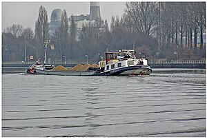
Waves in the Kelvin wake pattern generated by a ship on the Maas–Waalkanaal in The Netherlands. The transverse waves in this Kelvin wake pattern are nearly plane Stokes waves.

NOAA ship Delaware II in bad weather on Georges Bank. While these ocean waves are random, and not Stokes waves (in the strict sense), they indicate the typical sharp crests and flat troughs as found in nonlinear surface gravity waves.

A fundamental problem in finding solutions for surface gravity waves is that boundary conditions have to be applied at the position of the free surface, which is not known beforehand and is thus a part of the solution to be found. Sir George Stokes solved this nonlinear wave problem in 1847 by expanding the relevant potential flow quantities in a Taylor series around the mean (or still) surface elevation. ^[12] As a result, the boundary conditions can be expressed in terms of quantities at the mean (or still) surface elevation (which is fixed and known).

Next, a solution for the nonlinear wave problem (including the Taylor series expansion around the mean or still surface elevation) is sought by means of a perturbation series – known as the Stokes expansion – in terms of a small parameter, most often the wave steepness. The unknown terms in the expansion can be solved sequentially. ^{[6] [8]} Often, only a small number of terms is needed to provide a solution of sufficient accuracy for engineering purposes. ^[11] Typical applications are in the design of coastal and offshore structures, and of ships.

Another property of nonlinear waves is that the phase speed of nonlinear waves depends on the wave height. In a perturbation-series approach, this easily gives rise to a spurious secular variation of the solution, in contradiction with the periodic behaviour of the waves. Stokes solved this problem by also expanding the dispersion relationship into a perturbation series, by a method now known as the Lindstedt–Poincaré method. ^[6]

Applicability

Validity of several theories for periodic water waves, according to Le Méhauté (1976). The light-blue area gives the range of validity of cnoidal wave theory; light-yellow for Airy wave theory; and the dashed blue lines demarcate between the required order in Stokes's wave theory. The light-gray shading gives the range extension by numerical approximations using fifth-order stream-function theory, for high waves (H > 1⁄4 H_breaking).

Stokes's wave theory, when using a low order of the perturbation expansion (e.g. up to second, third or fifth order), is valid for nonlinear waves on intermediate and deep water, that is for wavelengths (λ) not large as compared with the mean depth (h). In shallow water, the low-order Stokes expansion breaks down (gives unrealistic results) for appreciable wave amplitude (as compared to the depth). Then, Boussinesq approximations are more appropriate. Further approximations on Boussinesq-type (multi-directional) wave equations lead – for one-way wave propagation – to the Korteweg–de Vries equation or the Benjamin–Bona–Mahony equation. Like (near) exact Stokes-wave solutions, ^[14] these two equations have solitary wave (soliton) solutions, besides periodic-wave solutions known as cnoidal waves. ^[11]

Modern extensions

Already in 1914, Wilton extended the Stokes expansion for deep-water surface gravity waves to tenth order, although introducing errors at the eight order. ^[15] A fifth-order theory for finite depth was derived by De in 1955. ^[16] For engineering use, the fifth-order formulations of Fenton are convenient, applicable to both Stokes first and second definition of phase speed (celerity). ^[17] The demarcation between when fifth-order Stokes theory is preferable over fifth-order cnoidal wave theory is for Ursell parameters below about 40. ^{[10] [11]}

Different choices for the frame of reference and expansion parameters are possible in Stokes-like approaches to the nonlinear wave problem. In 1880, Stokes himself inverted the dependent and independent variables, by taking the velocity potential and stream function as the independent variables, and the coordinates (x,z) as the dependent variables, with x and z being the horizontal and vertical coordinates respectively. ^[18] This has the advantage that the free surface, in a frame of reference in which the wave is steady (i.e. moving with the phase velocity), corresponds with a line on which the stream function is a constant. Then the free surface location is known beforehand, and not an unknown part of the solution. The disadvantage is that the radius of convergence of the rephrased series expansion reduces. ^[19]

Another approach is by using the Lagrangian frame of reference, following the fluid parcels. The Lagrangian formulations show enhanced convergence, as compared to the formulations in both the Eulerian frame, and in the frame with the potential and streamfunction as independent variables. ^{[20] [21]}

An exact solution for nonlinear pure capillary waves of permanent form, and for infinite fluid depth, was obtained by Crapper in 1957. Note that these capillary waves – being short waves forced by surface tension, if gravity effects are negligible – have sharp troughs and flat crests. This contrasts with nonlinear surface gravity waves, which have sharp crests and flat troughs. ^[22]

Several integral properties of Stokes waves on deep water as a function of wave steepness. The wave steepness is defined as the ratio of wave height H to the wavelength λ. The wave properties are made dimensionless using the wavenumber k = 2π / λ, gravitational acceleration g and the fluid density ρ.
Shown are the kinetic energy density T, the potential energy density V, the total energy density E = T + V, the horizontal wave momentum density I, and the relative enhancement of the phase speed c. Wave energy densities T, V and E are integrated over depth and averaged over one wavelength, so they are energies per unit of horizontal area; the wave momentum density I is similar. The dashed black lines show 1/16 (kH) and 1/8 (kH) , being the values of the integral properties as derived from (linear) Airy wave theory. The maximum wave height occurs for a wave steepness H / λ ≈ 0.1412, above which no periodic surface gravity waves exist.
Note that the shown wave properties have a maximum for a wave height less than the maximum wave height (see e.g. Longuet-Higgins 1975; Cokelet 1977).

By use of computer models, the Stokes expansion for surface gravity waves has been continued, up to high (117th) order by Schwartz (1974). Schwartz has found that the amplitude a (or a₁) of the first-order fundamental reaches a maximum before the maximum wave height H is reached. Consequently, the wave steepness ka in terms of wave amplitude is not a monotone function up to the highest wave, and Schwartz utilizes instead kH as the expansion parameter. To estimate the highest wave in deep water, Schwartz has used Padé approximants and Domb–Sykes plots in order to improve the convergence of the Stokes expansion. Extended tables of Stokes waves on various depths, computed by a different method (but in accordance with the results by others), are provided in Williams ( 1981 , 1985 ).

Several exact relationships exist between integral properties – such as kinetic and potential energy, horizontal wave momentum and radiation stress – as found by Longuet-Higgins (1975). He shows, for deep-water waves, that many of these integral properties have a maximum before the maximum wave height is reached (in support of Schwartz's findings). Cokelet (1978) harvtxt error: no target: CITEREFCokelet1978 (help), using a method similar to the one of Schwartz, computed and tabulated integral properties for a wide range of finite water depths (all reaching maxima below the highest wave height). Further, these integral properties play an important role in the conservation laws for water waves, through Noether's theorem. ^[25]

In 2005, Hammack, Henderson and Segur have provided the first experimental evidence for the existence of three-dimensional progressive waves of permanent form in deep water – that is bi-periodic and two-dimensional progressive wave patterns of permanent form. ^[26] The existence of these three-dimensional steady deep-water waves has been revealed in 2002, from a bifurcation study of two-dimensional Stokes waves by Craig and Nicholls, using numerical methods. ^[27]

Convergence and instability

Convergence

Convergence of the Stokes expansion was first proved by Levi-Civita (1925) for the case of small-amplitude waves – on the free surface of a fluid of infinite depth. This was extended shortly afterwards by Struik (1926) for the case of finite depth and small-amplitude waves. ^[28]

Near the end of the 20th century, it was shown that for finite-amplitude waves the convergence of the Stokes expansion depends strongly on the formulation of the periodic wave problem. For instance, an inverse formulation of the periodic wave problem as used by Stokes – with the spatial coordinates as a function of velocity potential and stream function – does not converge for high-amplitude waves. While other formulations converge much more rapidly, e.g. in the Eulerian frame of reference (with the velocity potential or stream function as a function of the spatial coordinates). ^[19]

Highest wave

Stokes waves of maximum wave height on deep water, under the action of gravity.

The maximum wave steepness, for periodic and propagating deep-water waves, is H / λ = 0.1410633 ± 4 · 10⁻⁷, ^[29] so the wave height is about one-seventh (⁠1/7⁠) of the wavelength λ. ^[24] And surface gravity waves of this maximum height have a sharp wave crest – with an angle of 120° (in the fluid domain) – also for finite depth, as shown by Stokes in 1880. ^[18]

An accurate estimate of the highest wave steepness in deep water (H / λ ≈ 0.142) was already made in 1893, by John Henry Michell, using a numerical method. ^[30] A more detailed study of the behaviour of the highest wave near the sharp-cornered crest has been published by Malcolm A. Grant, in 1973. ^[31] The existence of the highest wave on deep water with a sharp-angled crest of 120° was proved by John Toland in 1978. ^[32] The convexity of η(x) between the successive maxima with a sharp-angled crest of 120° was independently proven by C.J. Amick et al. and Pavel I. Plotnikov in 1982 . ^{[33] [34]}

The highest Stokes wave – under the action of gravity – can be approximated with the following simple and accurate representation of the free surface elevation η(x,t): ^[35] $${\displaystyle {\frac {\eta }{\lambda }}=A\,\left[\cosh \,\left({\frac {x-ct}{\lambda }}\right)-1\right],}$$ with $${\displaystyle A={\frac {1}{{\sqrt {3}}\,\sinh \left({\frac {1}{2}}\right)}}\approx 1.108,}$$ for $${\displaystyle -{\tfrac {1}{2}}\,\lambda \leq (x-ct)\leq {\tfrac {1}{2}}\,\lambda ,}$$

and shifted horizontally over an integer number of wavelengths to represent the other waves in the regular wave train. This approximation is accurate to within 0.7% everywhere, as compared with the "exact" solution for the highest wave. ^[35]

Another accurate approximation – however less accurate than the previous one – of the fluid motion on the surface of the steepest wave is by analogy with the swing of a pendulum in a grandfather clock. ^[36]

Large library of Stokes waves computed with high precision for the case of infinite depth, represented with high accuracy (at least 27 digits after decimal point) as a Padé approximant can be found at StokesWave.org ^[37]

Instability

In deeper water, Stokes waves are unstable. ^[38] This was shown by T. Brooke Benjamin and Jim E. Feir in 1967. ^{[39] [40]} The Benjamin–Feir instability is a side-band or modulational instability, with the side-band modulations propagating in the same direction as the carrier wave; waves become unstable on deeper water for a relative depth kh > 1.363 (with k the wavenumber and h the mean water depth). ^[41] The Benjamin–Feir instability can be described with the nonlinear Schrödinger equation, by inserting a Stokes wave with side bands. ^[38] Subsequently, with a more refined analysis, it has been shown – theoretically and experimentally – that the Stokes wave and its side bands exhibit Fermi–Pasta–Ulam–Tsingou recurrence: a cyclic alternation between modulation and demodulation. ^[42]

In 1978 Longuet-Higgins, by means of numerical modelling of fully non-linear waves and modulations (propagating in the carrier wave direction), presented a detailed analysis of the region of instability in deep water: both for superharmonics (for perturbations at the spatial scales smaller than the wavelength ${\displaystyle \lambda }$) ^[43] and subharmonics (for perturbations at the spatial scales larger than ${\displaystyle \lambda }$). ^[44] With increase of Stokes wave's amplitude, new modes of superharmonic instability appear. Appearance of a new branch of instability happens when the energy of the wave passes extremum. Detailed analysis of the mechanism of appearance of the new branches of instability has shown that their behavior follows closely a simple law, which allows to find with a good accuracy instability growth rates for all known and predicted branches. ^[45] In Longuet-Higgins studies of two-dimensional wave motion, as well as the subsequent studies of three-dimensional modulations by McLean et al., new types of instabilities were found – these are associated with resonant wave interactions between five (or more) wave components. ^{[46] [47] [48]}

Stokes expansion

Governing equations for a potential flow

In many instances, the oscillatory flow in the fluid interior of surface waves can be described accurately using potential flow theory, apart from boundary layers near the free surface and bottom (where vorticity is important, due to viscous effects, see Stokes boundary layer). ^[49] Then, the flow velocity u can be described as the gradient of a velocity potential ${\displaystyle \Phi }$:

$${\displaystyle \mathbf {u} ={\boldsymbol {\nabla }}\Phi .}$$

(A)

Consequently, assuming incompressible flow, the velocity field u is divergence-free and the velocity potential ${\displaystyle \Phi }$ satisfies Laplace's equation ^[49]

$${\displaystyle \nabla ^{2}\Phi =0}$$

(B)

in the fluid interior.

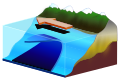
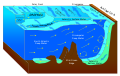
The fluid region is described using three-dimensional Cartesian coordinates (x,y,z), with x and y the horizontal coordinates, and z the vertical coordinate – with the positive z-direction opposing the direction of the gravitational acceleration. Time is denoted with t. The free surface is located at z = η(x,y,t), and the bottom of the fluid region is at z = −h(x,y).

The free-surface boundary conditions for surface gravity waves – using a potential flow description – consist of a kinematic and a dynamic boundary condition. ^[50] The kinematic boundary condition ensures that the normal component of the fluid's flow velocity, ${\displaystyle \mathbf {u} =[\partial \Phi /\partial x~~~\partial \Phi /\partial y~~~\partial \Phi /\partial z]^{\mathrm {T} }}$ in matrix notation, at the free surface equals the normal velocity component of the free-surface motion z = η(x,y,t):

$${\displaystyle {\frac {\partial \eta }{\partial t}}+{\frac {\partial \Phi }{\partial x}}\,{\frac {\partial \eta }{\partial x}}+{\frac {\partial \Phi }{\partial y}}\,{\frac {\partial \eta }{\partial y}}={\frac {\partial \Phi }{\partial z}}\qquad {\text{ at }}z=\eta (x,y,t).}$$

(C)

The dynamic boundary condition states that, without surface tension effects, the atmospheric pressure just above the free surface equals the fluid pressure just below the surface. For an unsteady potential flow this means that the Bernoulli equation is to be applied at the free surface. In case of a constant atmospheric pressure, the dynamic boundary condition becomes:

$${\displaystyle {\frac {\partial \Phi }{\partial t}}+{\tfrac {1}{2}}\,\left|\mathbf {u} \right|^{2}+g\,\eta =0\qquad {\text{ at }}z=\eta (x,y,t),}$$

(D)

where the constant atmospheric pressure has been taken equal to zero, without loss of generality.

Both boundary conditions contain the potential ${\displaystyle \Phi }$ as well as the surface elevation η. A (dynamic) boundary condition in terms of only the potential ${\displaystyle \Phi }$ can be constructed by taking the material derivative of the dynamic boundary condition, and using the kinematic boundary condition: ^{[49] [50] [51]} $${\displaystyle {\color {Gray}{{\Bigl (}{\frac {\partial }{\partial t}}+\mathbf {u} \cdot {\boldsymbol {\nabla }}{\Bigr )}\,\left({\frac {\partial \Phi }{\partial t}}+{\tfrac {1}{2}}\,|\mathbf {u} |^{2}+g\,\eta \right)=0}}}$$$${\displaystyle {\color {Gray}{\Rightarrow \quad {\frac {\partial ^{2}\Phi }{\partial t^{2}}}+g\,{\frac {\partial \Phi }{\partial z}}+\mathbf {u} \cdot {\boldsymbol {\nabla }}{\frac {\partial \Phi }{\partial t}}+{\tfrac {1}{2}}\,{\frac {\partial }{\partial t}}\left(|\mathbf {u} |^{2}\right)+{\tfrac {1}{2}}\,\mathbf {u} \cdot {\boldsymbol {\nabla }}\left(|\mathbf {u} |^{2}\right)=0}}}$$

$${\displaystyle {\color {Gray}{\Rightarrow \quad }}{\frac {\partial ^{2}\Phi }{\partial t^{2}}}+g\,{\frac {\partial \Phi }{\partial z}}+{\frac {\partial }{\partial t}}\left(|\mathbf {u} |^{2}\right)+{\tfrac {1}{2}}\,\mathbf {u} \cdot {\boldsymbol {\nabla }}\left(|\mathbf {u} |^{2}\right)=0\qquad {\text{ at }}z=\eta (x,y,t).}$$

(E)

At the bottom of the fluid layer, impermeability requires the normal component of the flow velocity to vanish: ^[49]

$${\displaystyle {\frac {\partial \Phi }{\partial n}}={\frac {1}{\sqrt {1+\left({\frac {\partial h}{\partial x}}\right)^{2}+\left({\frac {\partial h}{\partial y}}\right)^{2}}}}\,\left\{{\frac {\partial \Phi }{\partial z}}+{\frac {\partial h}{\partial x}}\,{\frac {\partial \Phi }{\partial x}}+{\frac {\partial h}{\partial y}}\,{\frac {\partial \Phi }{\partial y}}\right\}=0,\qquad {\text{ at }}z=-h(x,y),}$$

(F)

where h(x,y) is the depth of the bed below the datum z = 0 and n is the coordinate component in the direction normal to the bed.

For permanent waves above a horizontal bed, the mean depth h is a constant and the boundary condition at the bed becomes: $${\displaystyle {\frac {\partial \Phi }{\partial z}}=0\qquad {\text{ at }}z=-h.}$$

Taylor series in the free-surface boundary conditions

The free-surface boundary conditions (D) and (E) apply at the yet unknown free-surface elevation z = η(x,y,t). They can be transformed into boundary conditions at a fixed elevation z = constant by use of Taylor series expansions of the flow field around that elevation. ^[49] Without loss of generality the mean surface elevation – around which the Taylor series are developed – can be taken at z = 0. This assures the expansion is around an elevation in the proximity of the actual free-surface elevation. Convergence of the Taylor series for small-amplitude steady-wave motion was proved by Levi-Civita (1925).

The following notation is used: the Taylor series of some field f(x,y,z,t) around z = 0 – and evaluated at z = η(x,y,t) – is: ^[52] $${\displaystyle f(x,y,\eta ,t)=\left[f\right]_{0}+\eta \,\left[{\frac {\partial f}{\partial z}}\right]_{0}+{\frac {1}{2}}\,\eta ^{2}\,\left[{\frac {\partial ^{2}f}{\partial z^{2}}}\right]_{0}+\cdots }$$ with subscript zero meaning evaluation at z = 0, e.g.: [f]₀ = f(x,y,0,t).

Applying the Taylor expansion to free-surface boundary condition Eq. (E) in terms of the potential Φ gives: ^{[49] [52]}

$${\displaystyle {\begin{aligned}&\left[{\frac {\partial ^{2}\Phi }{\partial t^{2}}}+g\,{\frac {\partial \Phi }{\partial z}}\right]_{0}+\eta \left[{\frac {\partial }{\partial z}}\left({\frac {\partial ^{2}\Phi }{\partial t^{2}}}+g\,{\frac {\partial \Phi }{\partial z}}\right)\right]_{0}+\left[{\frac {\partial }{\partial t}}\left(|\mathbf {u} |^{2}\right)\right]_{0}\\&\quad +{\tfrac {1}{2}}\,\eta ^{2}\left[{\frac {\partial ^{2}}{\partial z^{2}}}\left({\frac {\partial ^{2}\Phi }{\partial t^{2}}}+g\,{\frac {\partial \Phi }{\partial z}}\right)\right]_{0}+\eta \left[{\frac {\partial ^{2}}{\partial t\,\partial z}}\left(|\mathbf {u} |^{2}\right)\right]_{0}+\left[{\tfrac {1}{2}}\,\mathbf {u} \cdot {\boldsymbol {\nabla }}\left(|\mathbf {u} |^{2}\right)\right]_{0}\\&\quad +\cdots =0,\end{aligned}}}$$

(G)

showing terms up to triple products of η, Φ and u, as required for the construction of the Stokes expansion up to third-order O((ka)³). Here, ka is the wave steepness, with k a characteristic wavenumber and a a characteristic wave amplitude for the problem under study. The fields η, Φ and u are assumed to be O(ka).

The dynamic free-surface boundary condition Eq. (D) can be evaluated in terms of quantities at z = 0 as: ^{[49] [52]}

$${\displaystyle {\begin{aligned}&\left[{\frac {\partial \Phi }{\partial t}}+g\,\eta \right]_{0}+\eta \left[{\frac {\partial ^{2}\Phi }{\partial t\,\partial z}}\right]_{0}+{\biggl [}{\tfrac {1}{2}}\,\left|\mathbf {u} \right|^{2}{\biggr ]}_{0}\\&\quad +{\tfrac {1}{2}}\,\eta ^{2}\left[{\frac {\partial ^{3}\Phi }{\partial t\,\partial z^{2}}}\right]_{0}+\eta \left[{\frac {\partial }{\partial z}}\left({\tfrac {1}{2}}\,\left|\mathbf {u} \right|^{2}\right)\right]_{0}+\cdots =0.\end{aligned}}}$$

(H)

The advantages of these Taylor-series expansions fully emerge in combination with a perturbation-series approach, for weakly non-linear waves (ka ≪ 1).

Perturbation-series approach

The perturbation series are in terms of a small ordering parameter ε ≪ 1 – which subsequently turns out to be proportional to (and of the order of) the wave slope ka, see the series solution in this section. ^[53] So, take ε = ka: $${\displaystyle {\begin{aligned}\eta &=\varepsilon \,\eta _{1}+\varepsilon ^{2}\,\eta _{2}+\varepsilon ^{3}\,\eta _{3}+\cdots ,\\\Phi &=\varepsilon \,\Phi _{1}+\varepsilon ^{2}\,\Phi _{2}+\varepsilon ^{3}\,\Phi _{3}+\cdots \quad {\text{and}}\\\mathbf {u} &=\varepsilon \,\mathbf {u} _{1}+\varepsilon ^{2}\,\mathbf {u} _{2}+\varepsilon ^{3}\,\mathbf {u} _{3}+\cdots .\end{aligned}}}$$

When applied in the flow equations, they should be valid independent of the particular value of ε. By equating in powers of ε, each term proportional to ε to a certain power has to equal to zero. As an example of how the perturbation-series approach works, consider the non-linear boundary condition (G) ; it becomes: ^[6] $${\displaystyle {\begin{aligned}&\varepsilon \,\left\{{\frac {\partial ^{2}\Phi _{1}}{\partial t^{2}}}+g\,{\frac {\partial \Phi _{1}}{\partial z}}\right\}\\&+\varepsilon ^{2}\,\left\{{\frac {\partial ^{2}\Phi _{2}}{\partial t^{2}}}+g\,{\frac {\partial \Phi _{2}}{\partial z}}+\eta _{1}\,{\frac {\partial }{\partial z}}\left({\frac {\partial ^{2}\Phi _{1}}{\partial t^{2}}}+g\,{\frac {\partial \Phi _{1}}{\partial z}}\right)+{\frac {\partial }{\partial t}}\left(|\mathbf {u} _{1}|^{2}\right)\right\}\\&+\varepsilon ^{3}\,\left\{{\frac {\partial ^{2}\Phi _{3}}{\partial t^{2}}}+g\,{\frac {\partial \Phi _{3}}{\partial z}}+\eta _{1}\,{\frac {\partial }{\partial z}}\left({\frac {\partial ^{2}\Phi _{2}}{\partial t^{2}}}+g\,{\frac {\partial \Phi _{2}}{\partial z}}\right)\right.\\&\qquad \quad \left.+\eta _{2}\,{\frac {\partial }{\partial z}}\left({\frac {\partial ^{2}\Phi _{1}}{\partial t^{2}}}+g\,{\frac {\partial \Phi _{1}}{\partial z}}\right)+2\,{\frac {\partial }{\partial t}}\left(\mathbf {u} _{1}\cdot \mathbf {u} _{2}\right)\right.\\&\qquad \quad \left.+{\tfrac {1}{2}}\,\eta _{1}^{2}\,{\frac {\partial ^{2}}{\partial z^{2}}}\left({\frac {\partial ^{2}\Phi _{1}}{\partial t^{2}}}+g\,{\frac {\partial \Phi _{1}}{\partial z}}\right)+\eta _{1}\,{\frac {\partial ^{2}}{\partial t\,\partial z}}\left(|\mathbf {u} _{1}|^{2}\right)+{\tfrac {1}{2}}\,\mathbf {u} _{1}\cdot {\boldsymbol {\nabla }}\left(|\mathbf {u} _{1}|^{2}\right)\right\}\\&+{\mathcal {O}}\left(\varepsilon ^{4}\right)=0,\qquad {\text{at }}z=0.\end{aligned}}}$$

The resulting boundary conditions at z = 0 for the first three orders are:

First order:

$${\displaystyle {\frac {\partial ^{2}\Phi _{1}}{\partial t^{2}}}+g\,{\frac {\partial \Phi _{1}}{\partial z}}=0,}$$

(J1)

Second order:

$${\displaystyle {\frac {\partial ^{2}\Phi _{2}}{\partial t^{2}}}+g\,{\frac {\partial \Phi _{2}}{\partial z}}=-\eta _{1}\,{\frac {\partial }{\partial z}}\left({\frac {\partial ^{2}\Phi _{1}}{\partial t^{2}}}+g\,{\frac {\partial \Phi _{1}}{\partial z}}\right)-{\frac {\partial }{\partial t}}\left(|\mathbf {u} _{1}|^{2}\right),}$$

(J2)

Third order:

$${\displaystyle {\begin{aligned}{\frac {\partial ^{2}\Phi _{3}}{\partial t^{2}}}+g\,{\frac {\partial \Phi _{3}}{\partial z}}=&-\eta _{1}\,{\frac {\partial }{\partial z}}\left({\frac {\partial ^{2}\Phi _{2}}{\partial t^{2}}}+g\,{\frac {\partial \Phi _{2}}{\partial z}}\right)-\eta _{2}\,{\frac {\partial }{\partial z}}\left({\frac {\partial ^{2}\Phi _{1}}{\partial t^{2}}}+g\,{\frac {\partial \Phi _{1}}{\partial z}}\right)\\&-2\,{\frac {\partial }{\partial t}}\left(\mathbf {u} _{1}\cdot \mathbf {u} _{2}\right)-{\tfrac {1}{2}}\,\eta _{1}^{2}\,{\frac {\partial ^{2}}{\partial z^{2}}}\left({\frac {\partial ^{2}\Phi _{1}}{\partial t^{2}}}+g\,{\frac {\partial \Phi _{1}}{\partial z}}\right)\\&-\eta _{1}\,{\frac {\partial ^{2}}{\partial t\,\partial z}}\left(|\mathbf {u} _{1}|^{2}\right)-{\tfrac {1}{2}}\,\mathbf {u} _{1}\cdot {\boldsymbol {\nabla }}\left(|\mathbf {u} _{1}|^{2}\right).\end{aligned}}}$$

(J3)

In a similar fashion – from the dynamic boundary condition (H) – the conditions at z = 0 at the orders 1, 2 and 3 become:

First order:

$${\displaystyle {\frac {\partial \Phi _{1}}{\partial t}}+g\,\eta _{1}=0,}$$

(K1)

Second order:

$${\displaystyle {\frac {\partial \Phi _{2}}{\partial t}}+g\,\eta _{2}=-\eta _{1}\,{\frac {\partial ^{2}\Phi _{1}}{\partial t\,\partial z}}-{\tfrac {1}{2}}\,\left|\mathbf {u} _{1}\right|^{2},}$$

(K2)

Third order:

$${\displaystyle {\begin{aligned}{\frac {\partial \Phi _{3}}{\partial t}}+g\,\eta _{3}=&-\eta _{1}\,{\frac {\partial ^{2}\Phi _{2}}{\partial t\,\partial z}}-\eta _{2}\,{\frac {\partial ^{2}\Phi _{1}}{\partial t\,\partial z}}-\mathbf {u} _{1}\cdot \mathbf {u} _{2}\\&-{\tfrac {1}{2}}\,\eta _{1}^{2}\,{\frac {\partial ^{3}\Phi _{1}}{\partial t\,\partial z^{2}}}-\eta _{1}\,{\frac {\partial }{\partial z}}\left({\tfrac {1}{2}}\,\left|\mathbf {u} _{1}\right|^{2}\right).\end{aligned}}}$$

(K3)

For the linear equations (A) , (B) and (F) the perturbation technique results in a series of equations independent of the perturbation solutions at other orders:

$${\displaystyle \left.{\begin{array}{rcl}\mathbf {u} _{j}&=&{\boldsymbol {\nabla }}\Phi _{j},\\[1ex]\nabla ^{2}\Phi _{j}&=&0,\\[1ex]\displaystyle {\frac {\partial \Phi _{j}}{\partial n}}&=&0\quad {\text{ at }}z=-h,\end{array}}\right\}\qquad {\text{for all orders }}j\in \mathbb {N} ^{+}.}$$

(L)

The above perturbation equations can be solved sequentially, i.e. starting with first order, thereafter continuing with the second order, third order, etc.

Application to progressive periodic waves of permanent form

Animation of steep Stokes waves in deep water, with a wavelength of about twice the water depth, for three successive wave periods. The wave height is about 9.2% of the wavelength.
Description of the animation: The white dots are fluid particles, followed in time. In the case shown here, the mean Eulerian horizontal velocity below the wave trough is zero.

The waves of permanent form propagate with a constant phase velocity (or celerity), denoted as c. If the steady wave motion is in the horizontal x-direction, the flow quantities η and u are not separately dependent on x and time t, but are functions of x − ct: ^[55] $${\displaystyle \eta (x,t)=\eta (x-ct)\quad {\text{and}}\quad \mathbf {u} (x,z,t)=\mathbf {u} (x-ct,z).}$$

Further the waves are periodic – and because they are also of permanent form – both in horizontal space x and in time t, with wavelength λ and period τ respectively. Note that Φ(x,z,t) itself is not necessary periodic due to the possibility of a constant (linear) drift in x and/or t: ^[56] $${\displaystyle \Phi (x,z,t)=\beta x-\gamma t+\varphi (x-ct,z),}$$ with φ(x,z,t) – as well as the derivatives ∂Φ/∂t and ∂Φ/∂x – being periodic. Here β is the mean flow velocity below trough level, and γ is related to the hydraulic head as observed in a frame of reference moving with the wave's phase velocity c (so the flow becomes steady in this reference frame).

In order to apply the Stokes expansion to progressive periodic waves, it is advantageous to describe them through Fourier series as a function of the wave phase θ(x,t): ^{[48] [56]} $${\displaystyle \theta =kx-\omega t=k\left(x-ct\right),}$$

assuming waves propagating in the x–direction. Here k = 2π / λ is the wavenumber, ω = 2π / τ is the angular frequency and c = ω / k (= λ / τ) is the phase velocity.

Now, the free surface elevation η(x,t) of a periodic wave can be described as the Fourier series: ^{[11] [56]} $${\displaystyle \eta =\sum _{n=1}^{\infty }A_{n}\,\cos \,(n\theta ).}$$

Similarly, the corresponding expression for the velocity potential Φ(x,z,t) is: ^[56] $${\displaystyle \Phi =\beta x-\gamma t+\sum _{n=1}^{\infty }B_{n}\,{\biggl [}\cosh \,\left(nk\,(z+h)\right){\biggr ]}\,\sin \,(n\theta ),}$$

satisfying both the Laplace equation ∇²Φ = 0 in the fluid interior, as well as the boundary condition ∂Φ/∂z = 0 at the bed z = −h.

For a given value of the wavenumber k, the parameters: A_n, B_n (with n = 1, 2, 3, ...), c, β and γ have yet to be determined. They all can be expanded as perturbation series in ε. Fenton (1990) provides these values for fifth-order Stokes's wave theory.

For progressive periodic waves, derivatives with respect to x and t of functions f(θ,z) of θ(x,t) can be expressed as derivatives with respect to θ: $${\displaystyle {\frac {\partial f}{\partial x}}=+k\,{\frac {\partial f}{\partial \theta }}\qquad {\text{and}}\qquad {\frac {\partial f}{\partial t}}=-\omega \,{\frac {\partial f}{\partial \theta }}.}$$

The important point for non-linear waves – in contrast to linear Airy wave theory – is that the phase velocity c also depends on the wave amplitude a, besides its dependence on wavelength λ = 2π / k and mean depth h. Negligence of the dependence of c on wave amplitude results in the appearance of secular terms, in the higher-order contributions to the perturbation-series solution. Stokes (1847) already applied the required non-linear correction to the phase speed c in order to prevent secular behaviour. A general approach to do so is now known as the Lindstedt–Poincaré method. Since the wavenumber k is given and thus fixed, the non-linear behaviour of the phase velocity c = ω / k is brought into account by also expanding the angular frequency ω into a perturbation series: ^[9] $${\displaystyle \omega =\omega _{0}+\varepsilon \,\omega _{1}+\varepsilon ^{2}\,\omega _{2}+\cdots .}$$

Here ω₀ will turn out to be related to the wavenumber k through the linear dispersion relation. However time derivatives, through ∂f/∂t = −ω ∂f/∂θ, now also give contributions – containing ω₁, ω₂, etc. – to the governing equations at higher orders in the perturbation series. By tuning ω₁, ω₂, etc., secular behaviour can be prevented. For surface gravity waves, it is found that ω₁ = 0 and the first non-zero contribution to the dispersion relation comes from ω₂ (see e.g. the sub-section "Third-order dispersion relation" above). ^[9]

Stokes's two definitions of wave celerity

For non-linear surface waves there is, in general, ambiguity in splitting the total motion into a wave part and a mean part. As a consequence, there is some freedom in choosing the phase speed (celerity) of the wave. Stokes (1847) identified two logical definitions of phase speed, known as Stokes's first and second definition of wave celerity: ^{[6] [11] [57]}

1. Stokes's first definition of wave celerity has, for a pure wave motion, the mean value of the horizontal Eulerian flow-velocity Ū_E at any location below trough level equal to zero. Due to the irrotationality of potential flow, together with the horizontal sea bed and periodicity the mean horizontal velocity, the mean horizontal velocity is a constant between bed and trough level. So in Stokes first definition the wave is considered from a frame of reference moving with the mean horizontal velocity Ū_E. This is an advantageous approach when the mean Eulerian flow velocity Ū_E is known, e.g. from measurements.
2. Stokes's second definition of wave celerity is for a frame of reference where the mean horizontal mass transport of the wave motion equal to zero. This is different from the first definition due to the mass transport in the splash zone, i.e. between the trough and crest level, in the wave propagation direction. This wave-induced mass transport is caused by the positive correlation between surface elevation and horizontal velocity. In the reference frame for Stokes's second definition, the wave-induced mass transport is compensated by an opposing undertow (so Ū_E < 0 for waves propagating in the positive x-direction). This is the logical definition for waves generated in a wave flume in the laboratory, or waves moving perpendicular towards a beach.

As pointed out by Michael E. McIntyre, the mean horizontal mass transport will be (near) zero for a wave group approaching into still water, with also in deep water the mass transport caused by the waves balanced by an opposite mass transport in a return flow (undertow). ^[58] This is due to the fact that otherwise a large mean force will be needed to accelerate the body of water into which the wave group is propagating.

Notes

1. Figure 5 in: Susan Bartsch-Winkler; David K. Lynch (1988), "Catalog of worldwide tidal bore occurrences and characteristics", USGS Report (Circular 1022), U. S. Geological Survey: 12, Bibcode:1988usgs.rept...12B
2. Chakrabarti, S.K. (2005), Handbook of Offshore Engineering, Elsevier, p. 235, ISBN   9780080445687
3. Grant, M.A. (1973), "Standing Stokes waves of maximum height", Journal of Fluid Mechanics, 60 (3): 593–604, Bibcode:1973JFM....60..593G, doi:10.1017/S0022112073000364, S2CID   123179735
4. Ochi, Michel K. (2003), Hurricane-generated seas, Elsevier, p. 119, ISBN   9780080443126
5. Tayfun, M.A. (1980), "Narrow-band nonlinear sea waves", Journal of Geophysical Research, 85 (C3): 1548–1552, Bibcode:1980JGR....85.1548T, doi:10.1029/JC085iC03p01548
6. Dingemans, M.W. (1997), "Water wave propagation over uneven bottoms", NASA Sti/Recon Technical Report N, Advanced Series on Ocean Engineering, 13: 171–184, §2.8, Bibcode:1985STIN...8525769K, ISBN   978-981-02-0427-3, OCLC   36126836
7. Svendsen, I.A. (2006), Introduction to nearshore hydrodynamics, World Scientific, p. 370, ISBN   9789812561428
8. Toba, Yoshiaki (2003), Ocean–atmosphere interactions, Springer, pp. 27–31, ISBN   9781402011719
9. Whitham (1974 , pp. 471–476, §13.13)
10. Hedges, T.S. (1995), "Regions of validity of analytical wave theories", Proceedings of the Institution of Civil Engineers - Water Maritime and Energy, 112 (2): 111–114, doi:10.1680/iwtme.1995.27656
11. Fenton (1990)
12. Stokes (1847)
13. Le Méhauté, B. (1976), An introduction to hydrodynamics and water waves, Springer, ISBN   978-0387072326
14. Longuet-Higgins, M.S.; Fenton, J.D. (1974), "On the mass, momentum, energy and circulation of a solitary wave. II", Proceedings of the Royal Society A , 340 (1623): 471–493, Bibcode:1974RSPSA.340..471L, doi:10.1098/rspa.1974.0166, S2CID   124253945
15. Wilton (1914)
16. De (1955)
17. Fenton (1985), also (including corrections) in Fenton (1990)
18. Stokes (1880b)
19. Drennan, W.M.; Hui, W.H.; Tenti, G. (1992), "Accurate calculations of Stokes water waves of large amplitude", Zeitschrift für Angewandte Mathematik und Physik, 43 (2): 367–384, Bibcode:1992ZaMP...43..367D, doi:10.1007/BF00946637, S2CID   121134205
20. Buldakov, E.V.; Taylor, P.H.; Eatock Taylor, R. (2006), "New asymptotic description of nonlinear water waves in Lagrangian coordinates", Journal of Fluid Mechanics, 562: 431–444, Bibcode:2006JFM...562..431B, CiteSeerX   10.1.1.492.5377 , doi:10.1017/S0022112006001443 (inactive 2 December 2024), S2CID   29506471
21. Clamond, D. (2007), "On the Lagrangian description of steady surface gravity waves", Journal of Fluid Mechanics, 589: 433–454, Bibcode:2007JFM...589..433C, CiteSeerX   10.1.1.526.5643 , doi:10.1017/S0022112007007811, S2CID   123255841
22. Crapper (1957)
23. This figure is a remake and adaptation of Figure 1 in Schwartz & Fenton (1982)
24. Schwartz & Fenton (1982)
25. Benjamin, T.B.; Olver, P.J. (1982), "Hamiltonian structure, symmetries and conservation laws for water waves", Journal of Fluid Mechanics, 125: 137–185, Bibcode:1982JFM...125..137B, doi:10.1017/S0022112082003292 (inactive 2 December 2024), S2CID   11744174
26. Hammack, J.L.; Henderson, D.M.; Segur, H. (2005), "Progressive waves with persistent two-dimensional surface patterns in deep water", Journal of Fluid Mechanics, 532: 1–52, Bibcode:2005JFM...532....1H, doi:10.1017/S0022112005003733 (inactive 2 December 2024), S2CID   53416586
27. Craig, W.; Nicholls, D.P. (2002), "Traveling gravity water waves in two and three dimensions", European Journal of Mechanics B, 21 (6): 615–641, Bibcode:2002EuJMB..21..615C, doi:10.1016/S0997-7546(02)01207-4
28. Debnath, L. (2005), Nonlinear partial differential equations for scientists and engineers, Birkhäuser, pp. 181 & 418–419, ISBN   9780817643232
29. Dyachenko, S.A.; Lushnikov, P.M.; Korotkevich, A.O. (2016), "Branch Cuts of Stokes Wave on Deep Water. Part I: Numerical Solution and Padé Approximation", Studies in Applied Mathematics, 137 (4): 419–472, arXiv: 1507.02784 , doi:10.1111/sapm.12128, S2CID   52104285
30. Michell, J.H. (1893), "The highest waves in water", Philosophical Magazine, Series 5, 36 (222): 430–437, doi:10.1080/14786449308620499
31. Grant, Malcolm A. (1973), "The singularity at the crest of a finite amplitude progressive Stokes wave", Journal of Fluid Mechanics, 59 (2): 257–262, Bibcode:1973JFM....59..257G, doi:10.1017/S0022112073001552, S2CID   119356016
32. Toland, J.F. (1978), "On the existence of a wave of greatest height and Stokes's conjecture", Proceedings of the Royal Society A , 363 (1715): 469–485, Bibcode:1978RSPSA.363..469T, doi:10.1098/rspa.1978.0178, S2CID   120444295
33. Plotnikov, P.I. (1982), "A proof of the Stokes conjecture in the theory of surface waves.", Dinamika Splosh. Sredy [in Russian], 57: 41–76

    Reprinted in: Plotnikov, P.I. (2002), "A proof of the Stokes conjecture in the theory of surface waves.", Studies in Applied Mathematics , 3 (2): 217–244, doi:10.1111/1467-9590.01408

34. Amick, C.J.; Fraenkel, L.E.; Toland, J.F. (1982), "On the Stokes conjecture for the wave of extreme form", Acta Mathematica , 148: 193–214, doi: 10.1007/BF02392728
35. Rainey, R.C.T.; Longuet-Higgins, M.S. (2006), "A close one-term approximation to the highest Stokes wave on deep water", Ocean Engineering, 33 (14–15): 2012–2024, Bibcode:2006OcEng..33.2012R, doi:10.1016/j.oceaneng.2005.09.014
36. Longuet-Higgins, M.S. (1979), "Why is a water wave like a grandfather clock?", Physics of Fluids, 22 (9): 1828–1829, Bibcode:1979PhFl...22.1828L, doi: 10.1063/1.862789
37. Dyachenko, S.A.; Korotkevich, A.O.; Lushnikov, P.M.; Semenova, A.A.; Silantyev, D.A. (2013–2022), StokesWave.org
38. For a review of the instability of Stokes waves see e.g.:
    Craik, A.D.D. (1988), Wave interactions and fluid flows, Cambridge University Press, pp. 199–219, ISBN   978-0-521-36829-2
39. Benjamin, T. Brooke; Feir, J.E. (1967), "The disintegration of wave trains on deep water. Part 1. Theory", Journal of Fluid Mechanics, 27 (3): 417–430, Bibcode:1967JFM....27..417B, doi:10.1017/S002211206700045X, S2CID   121996479
40. Zakharov, V.E.; Ostrovsky, L.A. (2009). "Modulation instability: The beginning" (PDF). Physica D. 238 (5): 540–548. Bibcode:2009PhyD..238..540Z. doi:10.1016/j.physd.2008.12.002.
41. Benjamin, T.B. (1967), "Instability of periodic wavetrains in nonlinear dispersive systems", Proceedings of the Royal Society A , 299 (1456): 59–76, Bibcode:1967RSPSA.299...59B, doi:10.1098/rspa.1967.0123, S2CID   121661209 Concluded with a discussion by Klaus Hasselmann.
42. Lake, B.M.; Yuen, H.C.; Rungaldier, H.; Ferguson, W.E. (1977), "Nonlinear deep-water waves: theory and experiment. Part 2. Evolution of a continuous wave train", Journal of Fluid Mechanics, 83 (1): 49–74, Bibcode:1977JFM....83...49L, doi:10.1017/S0022112077001037, S2CID   123014293
43. Longuet-Higgins, M.S. (1978), "The instabilities of gravity waves of finite amplitude in deep water. I. Superharmonics", Proceedings of the Royal Society A , 360 (1703): 471–488, Bibcode:1978RSPSA.360..471L, doi:10.1098/rspa.1978.0080, S2CID   202575377
44. Longuet-Higgins, M.S. (1978), "The instabilities of gravity waves of finite amplitude in deep water. II. Subharmonics", Proceedings of the Royal Society A , 360 (1703): 489–505, Bibcode:1978RSPSA.360..471L, doi:10.1098/rspa.1978.0080, S2CID   202575377
45. Korotkevich, A.O.; Lushnikov, P.M.; Semenova, A.; Dyachenko, S.A. (2022), "Superharmonic instability of stokes waves", Studies in Applied Mathematics, 150: 119–134, arXiv: 2206.00725 , doi:10.1111/sapm.12535, S2CID   249282423
46. McLean, J.W.; Ma, Y.C.; Martin, D.U.; Saffman, P.G.; Yuen, H.C. (1981), "Three-dimensional instability of finite-amplitude water waves" (PDF), Physical Review Letters, 46 (13): 817–820, Bibcode:1981PhRvL..46..817M, doi:10.1103/PhysRevLett.46.817
47. McLean, J.W. (1982), "Instabilities of finite-amplitude water waves", Journal of Fluid Mechanics, 114: 315–330, Bibcode:1982JFM...114..315M, doi:10.1017/S0022112082000172 (inactive 2 December 2024), S2CID   122511104
48. Dias & Kharif (1999)
49. Phillips, O.M. (1980), Dynamics of the upper ocean (2nd ed.), Cambridge University Press, pp. 33–37, ISBN   978-0-521-29801-8
50. Mei (1989 , pp. 4–6)
51. Longuet-Higgins, M.S. (1962), "Resonant interactions between two trains of gravity waves", Journal of Fluid Mechanics, 12 (3): 321–332, Bibcode:1962JFM....12..321L, doi:10.1017/S0022112062000233, S2CID   122810532
52. Mei (1989 , pp. 607–608)
53. By non-dimensionalization of the flow equations and boundary conditions, different regimes may be identified, depending on the scaling of the coordinates and flow quantities. In deep(er) water, the characteristic wavelength is the only length scale available. So, the horizontal and vertical coordinates are all non-dimensionalized with the wavelength. This leads to Stokes wave theory. However, in shallow water, the water depth is the appropriate characteristic scale to make the vertical coordinate non-dimensional, while the horizontal coordinates are scaled with the wavelength – resulting in the Boussinesq approximation. For a discussion, see:
    • Beji, S. (1995), "Note on a nonlinearity parameter of surface waves", Coastal Engineering, 25 (1–2): 81–85, Bibcode:1995CoasE..25...81B, doi:10.1016/0378-3839(94)00031-R ;
    • Kirby, J.T. (1998), "Discussion of 'Note on a nonlinearity parameter of surface waves' by S. Beji", Coastal Engineering, 34 (1–2): 163–168, Bibcode:1998CoasE..34..163K, doi:10.1016/S0378-3839(98)00024-6 and
    • Beji, S. (1998), "Author's closure to J.T. Kirby's discussion 'Note on a nonlinearity parameter of surface waves'", Coastal Engineering, 34 (1–2): 169–171, Bibcode:1998CoasE..34..169B, doi:10.1016/S0378-3839(98)00018-0
54. The wave physics are computed with the Rienecker & Fenton (R&F) streamfunction theory. For a computer code to compute these see: Fenton, J.D. (1988), "The numerical solution of steady water wave problems", Computers & Geosciences, 14 (3): 357–368, Bibcode:1988CG.....14..357F, doi:10.1016/0098-3004(88)90066-0. The animations are made from the R&F results with a series of Matlab scripts and shell scripts.
55. Wehausen & Laitone (1960 , pp. 653–667, §27)
56. Whitham (1974 , pp. 553–556, §16.6)
57. Sarpkaya, Turgut; Isaacson, Michael (1981), Mechanics of wave forces on offshore structures, Van Nostrand Reinhold, p. 183, ISBN   9780442254025
58. McIntyre, M.E. (1981), "On the 'wave momentum' myth", Journal of Fluid Mechanics, 106: 331–347, Bibcode:1981JFM...106..331M, doi:10.1017/S0022112081001626 (inactive 29 November 2024), S2CID   18232994

References

By Sir George Gabriel Stokes

• Stokes, G.G. (1847), "On the theory of oscillatory waves", Transactions of the Cambridge Philosophical Society, 8: 441–455.
  

Reprinted in: Stokes, G.G. (1880a), "On the theory of oscillatory waves", Mathematical and Physical Papers, Volume I, Cambridge University Press, pp. 197–229, ISBN   9781001435534, OCLC   314316422

• Stokes, G.G. (1880b), "Supplement to a paper on the theory of oscillatory waves", Mathematical and Physical Papers, Volume I, Cambridge University Press, pp. 314–326, ISBN   9781001435534, OCLC   314316422

Other historical references

• Crapper, G.D. (1957), "An exact solution for progressive capillary waves of arbitrary amplitude", Journal of Fluid Mechanics, 2 (6): 532–540, Bibcode:1957JFM.....2..532C, doi:10.1017/S0022112057000348 (inactive 2 December 2024), S2CID   120377950
• De, S.C. (1955), "Contributions to the theory of Stokes waves", Mathematical Proceedings of the Cambridge Philosophical Society, 51 (4): 713–736, Bibcode:1955PCPS...51..713D, doi:10.1017/S0305004100030796, S2CID   122721263
• Levi-Civita, T. (1925), "Détermination rigoureuse des ondes permanentes d'ampleur finie", Mathematische Annalen, 93: 264–314, doi:10.1007/BF01449965, S2CID   121341503
• Struik, D.J. (1926), "Détermination rigoureuse des ondes irrotationelles périodiques dans un canal à profondeur finie", Mathematische Annalen, 95: 595–634, doi:10.1007/BF01206629, S2CID   122656179
• Lord Rayleigh (1917), "On periodic irrotational waves at the surface of deep water", Philosophical Magazine, Series 6, 33 (197): 381–389, doi:10.1080/14786440508635653.
  

Reprinted in: Strutt, John William (Lord Rayleigh) (1920), Scientific Papers, vol. 6, Cambridge University Press, pp. 478–485, §419, OCLC   2316730

• Wilton, J.R. (1914), "On deep water waves", Philosophical Magazine, Series 6, 27 (158): 385–394, doi:10.1080/14786440208635100

More recent (since 1960)

• Cokelet, E.D. (1977), "Steep gravity waves in water of arbitrary uniform depth", Philosophical Transactions of the Royal Society, 286 (1335): 183–230, Bibcode:1977RSPTA.286..183C, doi:10.1098/rsta.1977.0113, S2CID   119957640
• Craik, A.D.D. (2005), "George Gabriel Stokes on water wave theory", Annual Review of Fluid Mechanics, 37 (1): 23–42, Bibcode:2005AnRFM..37...23C, doi:10.1146/annurev.fluid.37.061903.175836
• Dias, F.; Kharif, C. (1999), "Nonlinear gravity and capillary–gravity waves", Annual Review of Fluid Mechanics, 31: 301–346, Bibcode:1999AnRFM..31..301D, doi:10.1146/annurev.fluid.31.1.301
• Fenton, J.D. (1985), "A fifth-order Stokes theory for steady waves", Journal of Waterway, Port, Coastal, and Ocean Engineering, 111 (2): 216–234, CiteSeerX   10.1.1.461.6157 , doi:10.1061/(ASCE)0733-950X(1985)111:2(216)
  

And in (including corrections):

Fenton, J.D. (1990), "Nonlinear wave theories", in LeMéhauté, B.; Hanes, D.M. (eds.), Ocean Engineering Science (PDF), The Sea, vol. 9A, Wiley Interscience, pp. 3–25, ISBN   9780674017399

• Longuet-Higgins, M.S. (1975), "Integral properties of periodic gravity waves of finite amplitude", Proceedings of the Royal Society A , 342 (1629): 157–174, Bibcode:1975RSPSA.342..157L, doi:10.1098/rspa.1975.0018, S2CID   123723040
• Mei, C.C. (1989), The Applied Dynamics of Ocean Surface Waves, World Scientific, ISBN   9789971507893
• Schwartz, L.W. (1974), "Computer extension and analytic continuation of Stokes's expansion for gravity waves", Journal of Fluid Mechanics, 62 (3): 553–578, Bibcode:1974JFM....62..553S, doi:10.1017/S0022112074000802 (inactive 2 December 2024), S2CID   120140832
• Schwartz, L.W.; Fenton, J.D. (1982), "Strongly nonlinear waves", Annual Review of Fluid Mechanics, 14: 39–60, Bibcode:1982AnRFM..14...39S, doi:10.1146/annurev.fl.14.010182.000351
• Wehausen, J. V. & Laitone, E. V. (1960), Flügge, S. & Truesdell, C. (eds.), "Surface Waves", Encyclopaedia of Physics, 9: 653–667, §27, OCLC   612422741
• Whitham, G.B. (1974), Linear and nonlinear waves, Wiley-Interscience, ISBN   978-0-471-94090-6
• Williams, J.M. (1981), "Limiting gravity waves in water of finite depth", Philosophical Transactions of the Royal Society, Series A, 302 (1466): 139–188, Bibcode:1981RSPTA.302..139W, doi:10.1098/rsta.1981.0159, S2CID   122673867 and
  

Williams, J.M. (1985), Tables of progressive gravity waves, Pitman, ISBN   978-0273087335

External links

• Jun Zhang, Stokes waves applet, Texas A&M University, retrieved 2012-08-09