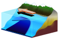
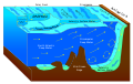
Geostrophic current

An example of a geostrophic flow in the Northern Hemisphere.

A northern-hemisphere gyre in geostrophic balance. Paler water is less dense than dark water, but more dense than air; the outwards pressure gradient is balanced by the 90 degrees-right-of-flow coriolis force. The structure will eventually dissipate due to friction and mixing of water properties.

A geostrophic current is an oceanic current in which the pressure gradient force is balanced by the Coriolis effect. The direction of geostrophic flow is parallel to the isobars, with the high pressure to the right of the flow in the Northern Hemisphere, and the high pressure to the left in the Southern Hemisphere. This concept is familiar from weather maps, whose isobars show the direction of geostrophic winds. Geostrophic flow may be either barotropic or baroclinic. A geostrophic current may also be thought of as a rotating shallow water wave with a frequency of zero.

The principle of geostrophy or geostrophic balance is useful to oceanographers because it allows them to infer ocean currents from measurements of the sea surface height (by combined satellite altimetry and gravimetry) or from vertical profiles of seawater density taken by ships or autonomous buoys. The major currents of the world's oceans, such as the Gulf Stream, the Kuroshio Current, the Agulhas Current, and the Antarctic Circumpolar Current, are all approximately in geostrophic balance and are examples of geostrophic currents.

Simple explanation

Sea water naturally tends to move from a region of high pressure (or high sea level) to a region of low pressure (or low sea level). The force pushing the water towards the low pressure region is called the pressure gradient force. In a geostrophic flow, instead of water moving from a region of high pressure (or high sea level) to a region of low pressure (or low sea level), it moves along the lines of equal pressure (isobars). This occurs because the Earth is rotating. The rotation of the earth results in a "force" being felt by the water moving from the high to the low, known as Coriolis force. The Coriolis force acts at right angles to the flow, and when it balances the pressure gradient force, the resulting flow is known as geostrophic.

As stated above, the direction of flow is with the high pressure to the right of the flow in the Northern Hemisphere, and the high pressure to the left in the Southern Hemisphere. The direction of the flow depends on the hemisphere, because the direction of the Coriolis force is opposite in the different hemispheres.

Formulation

See also: Geostrophic wind § Formulation

The geostrophic equations are a simplified form of the Navier–Stokes equations in a rotating reference frame. In particular, it is assumed that there is no acceleration (steady-state), that there is no viscosity, and that the pressure is hydrostatic. The resulting balance is (Gill, 1982):

${\displaystyle fv={\frac {1}{\rho }}{\frac {\partial p}{\partial x}}}$

${\displaystyle fu=-{\frac {1}{\rho }}{\frac {\partial p}{\partial y}}}$

where ${\displaystyle f}$ is the Coriolis parameter, ${\displaystyle \rho }$ is the density, ${\displaystyle p}$ is the pressure and ${\displaystyle u,v}$ are the velocities in the ${\displaystyle x,y}$-directions respectively.

One special property of the geostrophic equations, is that they satisfy the steady-state version of the continuity equation. That is:

${\displaystyle {\frac {\partial u}{\partial x}}+{\frac {\partial v}{\partial y}}=0}$

Rotating waves of zero frequency

The equations governing a linear, rotating shallow water wave are:

${\displaystyle {\frac {\partial u}{\partial t}}-fv=-{\frac {1}{\rho }}{\frac {\partial p}{\partial x}}}$

${\displaystyle {\frac {\partial v}{\partial t}}+fu=-{\frac {1}{\rho }}{\frac {\partial p}{\partial y}}}$

The assumption of steady-state made above (no acceleration) is:

${\displaystyle {\frac {\partial u}{\partial t}}={\frac {\partial v}{\partial t}}=0}$

Alternatively, we can assume a wave-like, periodic, dependence in time:

${\displaystyle u\propto v\propto e^{i\omega t}}$

In this case, if we set ${\displaystyle \omega =0}$, we have reverted to the geostrophic equations above. Thus a geostrophic current can be thought of as a rotating shallow water wave with a frequency of zero.

See also

• Oceans portal

• Geostrophic wind

References

• Gill, Adrian E. (1982), Atmosphere-Ocean Dynamics , International Geophysics Series, vol. 30, Oxford: Academic Press, ISBN   0-12-283522-0