A surface weather analysis for the United States on October 21, 2006.
A weather map, also known as synoptic weather chart, displays various meteorological features across a particular area at a particular point in time and has various symbols which all have specific meanings.[1] Such maps have been in use since the mid-19th century and are used for research and weather forecasting purposes. Maps using isotherms show temperature gradients,[2] which can help locate weather fronts. Isotach maps, analyzing lines of equal wind speed,[3] on a constant pressure surface of 300 or 250hPa show where the jet stream is located. Use of constant pressure charts at the 700 and 500hPa level can indicate tropical cyclone motion. Two-dimensional streamlines based on wind speeds at various levels show areas of convergence and divergence in the wind field, which are helpful in determining the location of features within the wind pattern. A popular type of surface weather map is the surface weather analysis, which plots isobars to depict areas of high pressure and low pressure. Cloud codes are translated into symbols and plotted on these maps along with other meteorological data that are included in synoptic reports sent by professionally trained observers.
The use of weather charts in a modern sense began in the middle portion of the 19th century in order to devise a theory on storm systems.[4] During the Crimean War a storm devastated the French fleet at Balaklava, and the French scientist Urbain Le Verrier was able to show that if a chronological map of the storm had been issued, the path it would take could have been predicted and avoided by the fleet.
In England, the scientist Francis Galton heard of this work, as well as the pioneering weather forecasts of Robert FitzRoy. After gathering information from weather stations across the country for the month of October 1861, he plotted the data on a map using his own system of symbols, thereby creating the world's first weather map. He used his map to prove that air circulated clockwise around areas of high pressure; he coined the term 'anticyclone' to describe the phenomenon. He was also instrumental in publishing the first weather map in a newspaper, for which he modified the pantograph (an instrument for copying drawings) to inscribe the map onto printing blocks. The Times began printing weather maps using these methods with data from the Meteorological Office.[5]
US weather map from 1843
The introduction of country-wide weather maps required the existence of national telegraph networks so that data from across the country could be gathered in real time and remain relevant for all analysis. The first such use of the telegraph for gathering data on the weather was the Manchester Examiner newspaper in 1847:[6]
...led us to inquire if the electric telegraph was yet extended far enough from Manchester to obtain information from the eastern counties...inquiries were made at the following places; and hypothesis were returned, which we append...
It was also important for time to be standardized across time zones so that the information on the map should accurately represent the weather at a given time. A standardized time system was first used to coordinate the British railway network in 1847, with the inauguration of Greenwich Mean Time.
In the US, The Smithsonian Institution developed its network of observers over much of the central and eastern United States between the 1840s and 1860s once Joseph Henry took the helm.[7] The U.S. Army Signal Corps inherited this network between 1870 and 1874 by an act of Congress, and expanded it to the west coast soon afterwards. At first, not all the data on the map was used due to a lack of time standardization. The United States fully adopted time zones in 1905, when Detroit finally established standard time.[8][9]
20th century
Light tables were important to the construction of surface weather analyses into the 1990s
The use of frontal zones on weather maps began in the 1910s in Norway. Polar front theory is attributed to Jacob Bjerknes, derived from a coastal network of observation sites in Norway during World War I. This theory proposed that the main inflow into a cyclone was concentrated along two lines of convergence, one ahead of the low and another trailing behind the low. The convergence line ahead of the low became known as either the steering line or the warm front. The trailing convergence zone was referred to as the squall line or cold front. Areas of clouds and rainfall appeared to be focused along these convergence zones. The concept of frontal zones led to the concept of air masses. The nature of the three-dimensional structure of the cyclone would wait for the development of the upper air network during the 1940s.[10] Since the leading edge of air mass changes bore resemblance to the military fronts of World War I, the term "front" came into use to represent these lines.[11] The United States began to formally analyze fronts on surface analyses in late 1942, when the WBAN Analysis Center opened in downtown Washington, D.C.[12]
In addition to surface weather maps, weather agencies began to generate constant pressure charts. In 1948, the United States began the Daily Weather Map series, which at first analyzed the 700 hPa level, which is around 3,000 metres (9,800ft) above sea level.[13] By May 14, 1954, the 500 hPa surface was being analyzed, which is about 5,520 metres (18,110ft) above sea level.[14] The effort to automate map plotting began in the United States in 1969,[15] with the process complete in the 1970s. A similar initiative was started in India by Indian Meteorological Department in 1969.[16]Hong Kong completed their process of automated surface plotting by 1987.[17]
By 1999, computer systems and software had finally become sophisticated enough to allow for the ability to underlay on the same workstation satellite imagery, radar imagery, and model-derived fields such as atmospheric thickness and frontogenesis in combination with surface observations to make for the best possible surface analysis. In the United States, this development was achieved when Intergraph workstations were replaced by n-AWIPS workstations.[18] By 2001, the various surface analyses done within the National Weather Service were combined into the Unified Surface Analysis, which is issued every six hours and combines the analyses of four different centers.[19] Recent advances in both the fields of meteorology and geographic information systems have made it possible to devise finely tailored products that take us from the traditional weather map into an entirely new realm. Weather information can quickly be matched to relevant geographical detail. For instance, icing conditions can be mapped onto the road network. This will likely continue to lead to changes in the way surface analyses are created and displayed over the next several years.[20]
Low étage (Sc,St) and upward-growing vertical (Cu, Cb)
Middle étage (Ac,As) and downward-growing vertical (Ns)
High étage (Ci,Cc,Cs)
Present weather symbols used on weather mapsWind barb interpretation
A station model is a symbolic illustration showing the weather occurring at a given reporting station. Meteorologists created the station model to plot a number of weather elements in a small space on weather maps. Maps filled with dense station-model plots can be difficult to read, but they allow meteorologists, pilots, and mariners to see important weather patterns. A computer draws a station model for each observation location. The station model is primarily used on surface-weather maps, but can also be used to show the weather aloft. A completed station-model map allows users to analyze patterns in air pressure, temperature, wind, cloud cover, and precipitation.[21]
Station model plots use an internationally accepted coding convention that has changed little since August 1, 1941. Elements in the plot show the key weather elements, including temperature, dewpoint, wind, cloud cover, air pressure, pressure tendency, and precipitation.[22][23] Winds have a standard notation when plotted on weather maps. More than a century ago, winds were plotted as arrows, with feathers on just one side depicting five knots of wind, while feathers on both sides depicted 10 knots (19km/h) of wind. The notation changed to that of half of an arrow, with half of a wind barb indicating five knots, a full barb ten knots, and a pennant flag fifty knots.
Because of the structure of the SYNOP code, a maximum of three cloud symbols can be plotted for each reporting station that appears on the weather map. All cloud types are coded and transmitted by trained observers then plotted on maps as low, middle, or high-étage using special symbols for each major cloud type. Any cloud type with significant vertical extent that can occupy more than one étage is coded as low (cumulus and cumulonimbus) or middle (nimbostratus) depending on the altitude level or étage where it normally initially forms aside from any vertical growth that takes place.[24][25] The symbol used on the map for each of these étages at a particular observation time is for the genus, species, variety, mutation, or cloud motion that is considered most important according to criteria set out by the World Meteorological Organization (WMO). If these elements for any étage at the time of observation are deemed to be of equal importance, then the type which is predominant in amount is coded by the observer and plotted on the weather map using the appropriate symbol. Special weather maps in aviation show areas of icing and turbulence.[26]
Types
Alaskan aviation weather map
Aviation maps
Aviation interests have their own set of weather maps. One type of map shows where VFR (visual flight rules) are in effect and where IFR (instrument flight rules) are in effect. Weather depiction plots show ceiling height (level where at least half the sky is covered with clouds) in hundreds of feet, present weather, and cloud cover.[27] Icing maps depict areas where icing can be a hazard for flying. Aviation-related maps also show areas of turbulence.[28]
Constant pressure charts
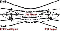
An upper-level jet streak. DIV areas are regions of divergence aloft, which usually leads to surface convergence and cyclogenesis
Constant pressure charts normally contain plotted values of temperature, humidity, wind, and the vertical height above sea level of the pressure surface.[29] They have a variety of uses. In the mountainous terrain of the western United States and Mexican Plateau, the 850 hPa pressure surface can be a more realistic depiction of the weather pattern than a standard surface analysis. Using the 850 and 700 hPa pressure surfaces, one can determine when and where warm advection (coincident with upward vertical motion) and cold advection (coincident with downward vertical motion) is occurring within the lower portions of the troposphere. Areas with small dewpoint depressions and are below freezing indicate the presence of icing conditions for aircraft.[30] The 500 hPa pressure surface can be used as a rough guide for the motion of many tropical cyclones. Shallower tropical cyclones, which have experienced vertical wind shear, tend to be steered by winds at the 700 hPa level.[31]
Use of the 300 and 200 hPa constant pressure charts can indicate the strength of systems in the lower troposphere, as stronger systems near the Earth's surface are reflected as stronger features at these levels of the atmosphere. Isotachs are drawn at these levels, which a lines of equal wind speed. They are helpful in finding maxima and minima in the wind pattern. Minima in the wind pattern aloft are favorable for tropical cyclogenesis. Maxima in the wind pattern at various levels of the atmosphere show locations of jet streams. Areas colder than −40°C (−40°F) indicate a lack of significant icing, as long as there is no active thunderstorm activity.[30]
A surface weather analysis is a type of weather map that depicts positions for high and low-pressure areas, as well as various types of synoptic scale systems such as frontal zones. Isotherms can be drawn on these maps, which are lines of equal temperature. Isotherms are drawn normally as solid lines at a preferred temperature interval.[2] They show temperature gradients, which can be useful in finding fronts, which are on the warm side of large temperature gradients. By plotting the freezing line, isotherms can be useful in determination of precipitation type. Mesoscale boundaries such as tropical cyclones, outflow boundaries and squall lines also are analyzed on surface weather analyses.
Isobaric analysis is performed on these maps, which involves the construction of lines of equal mean sea level pressure. The innermost closed lines indicate the positions of relative maxima and minima in the pressure field. The minima are called low-pressure areas while the maxima are called high-pressure areas. Highs are often shown as H's whereas lows are shown as L's. Elongated areas of low pressure, or troughs, are sometimes plotted as thick, brown dashed lines down the trough axis.[32] Isobars are commonly used to place surface boundaries from the horse latitudes poleward, while streamline analyses are used in the tropics.[33] A streamline analysis is a series of arrows oriented parallel to wind, showing wind motion within a certain geographic area. "C"s depict cyclonic flow or likely areas of low pressure, while "A"s depict anticyclonic flow or likely positions of high-pressure areas.[34] An area of confluent streamlines shows the location of shearlines within the tropics and subtropics.[19]
This page is based on this Wikipedia article Text is available under the CC BY-SA 4.0 license; additional terms may apply. Images, videos and audio are available under their respective licenses.


