Stokes problem

Stokes problem in a viscous fluid due to the harmonic oscillation of a plane rigid plate (bottom black edge). Velocity (blue line) and particle excursion (red dots) as a function of the distance to the wall.

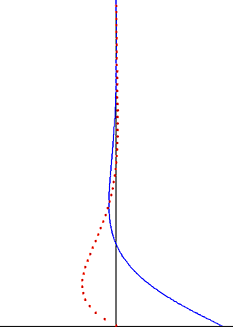
In fluid dynamics, Stokes problem also known as Stokes second problem or sometimes referred to as Stokes boundary layer or Oscillating boundary layer is a problem of determining the flow created by an oscillating solid surface, named after Sir George Stokes. This is considered one of the simplest unsteady problems that has an exact solution for the Navier-Stokes equations. ^{[1] [2]} In turbulent flow, this is still named a Stokes boundary layer, but now one has to rely on experiments, numerical simulations or approximate methods in order to obtain useful information on the flow.

Flow description ^{[3] [4]}

Consider an infinitely long plate which is oscillating with a velocity ${\displaystyle U\cos \omega t}$ in the ${\displaystyle x}$ direction, which is located at ${\displaystyle y=0}$ in an infinite domain of fluid, where ${\displaystyle \omega }$ is the frequency of the oscillations. The incompressible Navier-Stokes equations reduce to

${\displaystyle {\frac {\partial u}{\partial t}}=\nu {\frac {\partial ^{2}u}{\partial y^{2}}}}$

where ${\displaystyle \nu }$ is the kinematic viscosity. The pressure gradient does not enter into the problem. The initial, no-slip condition on the wall is

${\displaystyle u(0,t)=U\cos \omega t,\quad u(\infty ,t)=0,}$

and the second boundary condition is due to the fact that the motion at ${\displaystyle y=0}$ is not felt at infinity. The flow is only due to the motion of the plate, there is no imposed pressure gradient.

Solution ^{[5] [6]}

The initial condition is not required because of periodicity. Since both the equation and the boundary conditions are linear, the velocity can be written as the real part of some complex function

${\displaystyle u=U\Re \left[e^{i\omega t}f(y)\right]}$

because ${\displaystyle \cos \omega t=\Re e^{i\omega t}}$.

Substituting this into the partial differential equation reduces it to ordinary differential equation

${\displaystyle f''-{\frac {i\omega }{\nu }}f=0}$

with boundary conditions

${\displaystyle f(0)=1,\quad f(\infty )=0}$

The solution to the above problem is

${\displaystyle f(y)=\exp \left[-{\frac {1+i}{\sqrt {2}}}{\sqrt {\frac {\omega }{\nu }}}y\right]}$

${\displaystyle u(y,t)=Ue^{-{\sqrt {\frac {\omega }{2\nu }}}y}\cos \left(\omega t-{\sqrt {\frac {\omega }{2\nu }}}y\right)}$

The disturbance created by the oscillating plate travels as the transverse wave through the fluid, but it is highly damped by the exponential factor. The depth of penetration ${\displaystyle \delta ={\sqrt {2\nu /\omega }}}$ of this wave decreases with the frequency of the oscillation, but increases with the kinematic viscosity of the fluid.

The force per unit area exerted on the plate by the fluid is

${\displaystyle F=\mu \left({\frac {\partial u}{\partial y}}\right)_{y=0}={\sqrt {\rho \omega \mu }}U\cos \left(\omega t-{\frac {\pi }{4}}\right)}$

There is a phase shift between the oscillation of the plate and the force created.

Vorticity oscillations near the boundary

An important observation from Stokes' solution for the oscillating Stokes flow is that vorticity oscillations are confined to a thin boundary layer and damp exponentially when moving away from the wall. ^[7] This observation is also valid for the case of a turbulent boundary layer. Outside the Stokes boundary layer – which is often the bulk of the fluid volume – the vorticity oscillations may be neglected. To good approximation, the flow velocity oscillations are irrotational outside the boundary layer, and potential flow theory can be applied to the oscillatory part of the motion. This significantly simplifies the solution of these flow problems, and is often applied in the irrotational flow regions of sound waves and water waves.

Fluid bounded by an upper wall

If the fluid domain is bounded by an upper, stationary wall, located at a height ${\displaystyle y=h}$, the flow velocity is given by

${\displaystyle u(y,t)={\frac {U}{2(\cosh 2\lambda h-\cos 2\lambda h)}}[e^{-\lambda (y-2h)}\cos(\omega t-\lambda y)+e^{\lambda (y-2h)}\cos(\omega t+\lambda y)-e^{-\lambda y}\cos(\omega t-\lambda y+2\lambda h)-e^{\lambda y}\cos(\omega t+\lambda y-2\lambda h)]}$

where ${\displaystyle \lambda ={\sqrt {\omega /(2\nu )}}}$.

Fluid bounded by a free surface

Suppose the extent of the fluid domain be ${\displaystyle 0<y<h}$ with ${\displaystyle y=h}$ representing a free surface. Then the solution as shown by Chia-Shun Yih in 1968 ^[8] is given by

${\displaystyle u(y,t)={\frac {U\cos h/\delta \,\mathrm {cosh} \,h/\delta }{2(\cos ^{2}h/\delta +\mathrm {sinh} ^{2}h/\delta )}}\Re \left\{W+W^{*}-i\mathrm {tanh} \,h/\delta \,\tan h/\delta \,(W-W^{*})\right\},\qquad W=\mathrm {cosh} [(1+i)(h-y)/\delta ]e^{i\omega t}}$

where ${\displaystyle \delta ={\sqrt {2\nu /\omega }}.}$

Flow due to an oscillating pressure gradient near a plane rigid plate

Stokes boundary layer due to the sinusoidal oscillation of the far-field flow velocity. The horizontal velocity is the blue line, and the corresponding horizontal particle excursions are the red dots.

The case for an oscillating far-field flow, with the plate held at rest, can easily be constructed from the previous solution for an oscillating plate by using linear superposition of solutions. Consider a uniform velocity oscillation ${\displaystyle u(\infty ,t)=U_{\infty }\cos \omega t}$ far away from the plate and a vanishing velocity at the plate ${\displaystyle u(0,t)=0}$. Unlike the stationary fluid in the original problem, the pressure gradient here at infinity must be a harmonic function of time. The solution is then given by

${\displaystyle u(y,t)=U_{\infty }\left[\,\cos \omega t-{\text{e}}^{-{\sqrt {\frac {\omega }{2\nu }}}y}\,\cos \left(\omega t-{\sqrt {\frac {\omega }{2\nu }}}y\right)\right],}$

which is zero at the wall y = 0, corresponding with the no-slip condition for a wall at rest. This situation is often encountered in sound waves near a solid wall, or for the fluid motion near the sea bed in water waves. The vorticity, for the oscillating flow near a wall at rest, is equal to the vorticity in case of an oscillating plate but of opposite sign.

Stokes problem in cylindrical geometry

Torsional oscillation

Consider an infinitely long cylinder of radius ${\displaystyle a}$ exhibiting torsional oscillation with angular velocity ${\displaystyle \Omega \cos \omega t}$ where ${\displaystyle \omega }$ is the frequency. Then the velocity approaches after the initial transient phase to ^[9]

${\displaystyle v_{\theta }=a\Omega \ \Re \left[{\frac {K_{1}(r{\sqrt {i\omega /\nu }})}{K_{1}(a{\sqrt {i\omega /\nu }})}}e^{i\omega t}\right]}$

where ${\displaystyle K_{1}}$ is the modified Bessel function of the second kind. This solution can be expressed with real argument ^[10] as:

${\displaystyle {\begin{aligned}v_{\theta }\left(r,t\right)&=\Psi \left\lbrace \left[{\textrm {kei}}_{1}\left({\sqrt {R_{\omega }}}\right){\textrm {kei}}_{1}\left({\sqrt {R_{\omega }}}r\right)+{\textrm {ker}}_{1}\left({\sqrt {R_{\omega }}}\right){\textrm {ker}}_{1}\left({\sqrt {R_{\omega }}}r\right)\right]\cos \left(t\right)\right.\\&+\left.\left[{\textrm {kei}}_{1}\left({\sqrt {R_{\omega }}}\right){\textrm {ker}}_{1}\left({\sqrt {R_{\omega }}}r\right)-{\textrm {ker}}_{1}\left({\sqrt {R_{\omega }}}\right){\textrm {kei}}_{1}\left({\sqrt {R_{\omega }}}r\right)\right]\sin \left(t\right)\right\rbrace \\\end{aligned}}}$

where

${\displaystyle \Psi =\left[{\textrm {kei}}_{1}^{2}\left({\sqrt {R_{\omega }}}\right)+{\textrm {ker}}_{1}^{2}\left({\sqrt {R_{\omega }}}\right)\right]^{-1},}$

${\displaystyle \mathrm {kei} }$ and ${\displaystyle \mathrm {ker} }$ are Kelvin functions and ${\displaystyle R_{\omega }}$is to the dimensionless oscillatory Reynolds number defined as ${\displaystyle R_{\omega }=\omega a^{2}/\nu }$, being ${\displaystyle \nu }$ the kinematic viscosity.

Axial oscillation

If the cylinder oscillates in the axial direction with velocity ${\displaystyle U\cos \omega t}$, then the velocity field is

${\displaystyle u=U\ \Re \left[{\frac {K_{0}(r{\sqrt {i\omega /\nu }})}{K_{0}(a{\sqrt {i\omega /\nu }})}}e^{i\omega t}\right]}$

where ${\displaystyle K_{0}}$ is the modified Bessel function of the second kind.

Stokes-Couette flow ^[11]

In the Couette flow, instead of the translational motion of one of the plate, an oscillation of one plane will be executed. If we have a bottom wall at rest at ${\displaystyle y=0}$ and the upper wall at ${\displaystyle y=h}$ is executing an oscillatory motion with velocity ${\displaystyle U\cos \omega t}$, then the velocity field is given by

${\displaystyle u=U\ \Re \left\{{\frac {\sin ky}{\sin kh}}\right\},\quad {\text{where}}\quad k={\frac {1+i}{\sqrt {2}}}{\sqrt {\frac {\omega }{\nu }}}.}$

The frictional force per unit area on the moving plane is ${\displaystyle -\mu U\Re \{k\cot kh\}}$ and on the fixed plane is ${\displaystyle \mu U\Re \{k\csc kh\}}$.

See also

• Rayleigh problem

References

1. Wang, C. Y. (1991). "Exact solutions of the steady-state Navier-Stokes equations". Annual Review of Fluid Mechanics. 23: 159–177. Bibcode:1991AnRFM..23..159W. doi:10.1146/annurev.fl.23.010191.001111.
2. Landau & Lifshitz (1987), pp. 83–85.
3. Batchelor, George Keith. An introduction to fluid dynamics. Cambridge university press, 2000.
4. Lagerstrom, Paco Axel. Laminar flow theory. Princeton University Press, 1996.
5. Acheson, David J. Elementary fluid dynamics. Oxford University Press, 1990.
6. Landau, Lev Davidovich, and Evgenii Mikhailovich Lifshitz. "Fluid mechanics." (1987).
7. Phillips (1977), p. 46.
8. Yih, C. S. (1968). Instability of unsteady flows or configurations Part 1. Instability of a horizontal liquid layer on an oscillating plane. Journal of Fluid Mechanics, 31(4), 737-751.
9. Drazin, Philip G., and Norman Riley. The Navier–Stokes equations: a classification of flows and exact solutions. No. 334. Cambridge University Press, 2006.
10. Rivero, M.; Garzón, F.; Núñez, J.; Figueroa, A. (2019). "Study of the flow induced by circular cylinder performing torsional oscillation". European Journal of Mechanics - B/Fluids. 78: 245–251. doi:10.1016/j.euromechflu.2019.08.002. S2CID   201253195.
11. Landau, L. D., & Sykes, J. B. (1987). Fluid Mechanics: Vol 6. pp. 88