Trochoidal wave

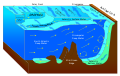
Surface elevation of a trochoidal wave (deep blue) propagating to the right. The trajectories of free surface particles are close circles (in cyan), and the flow velocity is shown in red, for the black particles. The wave height – difference between the crest and trough elevation – is denoted as ${\displaystyle H}$, the wavelength as ${\displaystyle \lambda }$ and the phase speed as ${\displaystyle c.}$

In fluid dynamics, a trochoidal wave or Gerstner wave is an exact solution of the Euler equations for periodic surface gravity waves. It describes a progressive wave of permanent form on the surface of an incompressible fluid of infinite depth. The free surface of this wave solution is an inverted (upside-down) trochoid – with sharper crests and flat troughs. This wave solution was discovered by Gerstner in 1802, and rediscovered independently by Rankine in 1863.

The flow field associated with the trochoidal wave is not irrotational: it has vorticity. The vorticity is of such a specific strength and vertical distribution that the trajectories of the fluid parcels are closed circles. This is in contrast with the usual experimental observation of Stokes drift associated with the wave motion. Also the phase speed is independent of the trochoidal wave's amplitude, unlike other nonlinear wave-theories (like those of the Stokes wave and cnoidal wave) and observations. For these reasons – as well as for the fact that solutions for finite fluid depth are lacking – trochoidal waves are of limited use for engineering applications.

In computer graphics, the rendering of realistic-looking ocean waves can be done by use of so-called Gerstner waves. This is a multi-component and multi-directional extension of the traditional Gerstner wave, often using fast Fourier transforms to make (real-time) animation feasible. ^[1]

Description of classical trochoidal wave

Vector contributions from the gravitational force (medium gray) and the gradient of the pressure (black) come together in an amazing way to produce the uniform circular motion of the fluid particles. For uniform circular motion, the net force (light gray) has constant magnitude and always points towards the center of the circle. The fluid particles are colored according to their ${\displaystyle b}$ values. Since the pressure is a function only of ${\displaystyle b}$, the animation illustrates how the pressure gradient vectors are always perpendicular to the color bands, and their magnitudes are larger when the color bands are closer together.

Using a Lagrangian specification of the flow field, the motion of fluid parcels is – for a periodic wave on the surface of a fluid layer of infinite depth: ^[2]

$${\displaystyle {\begin{aligned}X(a,b,t)&=a+{\frac {e^{kb}}{k}}\sin \left(k(a+ct)\right),\\Y(a,b,t)&=b-{\frac {e^{kb}}{k}}\cos \left(k(a+ct)\right),\end{aligned}}}$$

where ${\displaystyle x=X(a,b,t)}$ and ${\displaystyle y=Y(a,b,t)}$ are the positions of the fluid parcels in the ${\displaystyle (x,y)}$ plane at time ${\displaystyle t}$, with ${\displaystyle x}$ the horizontal coordinate and ${\displaystyle y}$ the vertical coordinate (positive upward, in the direction opposing gravity). The Lagrangian coordinates ${\displaystyle (a,b)}$ label the fluid parcels, with ${\displaystyle (x,y)=(a,b)}$ the centres of the circular orbits – around which the corresponding fluid parcel moves with constant speed ${\displaystyle c\,\exp(kb).}$ Further ${\textstyle k=2\pi /\lambda }$ is the wavenumber (and ${\displaystyle \lambda }$ the wavelength), while ${\displaystyle c}$ is the phase speed with which the wave propagates in the ${\displaystyle x}$-direction. The phase speed satisfies the dispersion relation:

$${\displaystyle c^{2}={\frac {g}{k}},}$$

which is independent of the wave nonlinearity (i.e. does not depend on the wave height ${\displaystyle H}$), and this phase speed ${\displaystyle c}$ the same as for Airy's linear waves in deep water.

The free surface is a line of constant pressure, and is found to correspond with a line ${\displaystyle b=b_{s}}$, where ${\displaystyle b_{s}}$ is a (nonpositive) constant. For ${\displaystyle b_{s}=0}$ the highest waves occur, with a cusp-shaped crest. Note that the highest (irrotational) Stokes wave has a crest angle of 120°, instead of the 0° for the rotational trochoidal wave. ^[3]

The wave height of the trochoidal wave is ${\textstyle H={\frac {2}{k}}\exp(kb_{s}).}$ The wave is periodic in the ${\displaystyle x}$-direction, with wavelength ${\displaystyle \lambda$ ;} and also periodic in time with period ${\textstyle T=\lambda /c={\sqrt {2\pi \lambda /g}}.}$

The vorticity ${\displaystyle \varpi }$ under the trochoidal wave is: ^[2]

$${\displaystyle \varpi (a,b,t)=-{\frac {2kce^{2kb}}{1-e^{2kb}}},}$$

varying with Lagrangian elevation ${\displaystyle b}$ and diminishing rapidly with depth below the free surface.

In computer graphics

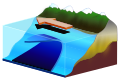
Animation (5 MB) of swell waves using multi-directional and multi-component Gerstner waves for the simulation of the ocean surface and POV-Ray for the 3D rendering. (The animation is periodic in time; it can be set to loop after right-clicking on it while it is playing).

A multi-component and multi-directional extension of the Lagrangian description of the free-surface motion – as used in Gerstner's trochoidal wave – is used in computer graphics for the simulation of ocean waves. ^[1] For the classical Gerstner wave the fluid motion exactly satisfies the nonlinear, incompressible and inviscid flow equations below the free surface. However, the extended Gerstner waves do in general not satisfy these flow equations exactly (although they satisfy them approximately, i.e. for the linearised Lagrangian description by potential flow). This description of the ocean can be programmed very efficiently by use of the fast Fourier transform (FFT). Moreover, the resulting ocean waves from this process look realistic, as a result of the nonlinear deformation of the free surface (due to the Lagrangian specification of the motion): sharper crests and flatter troughs.

The mathematical description of the free-surface in these Gerstner waves can be as follows: ^[1] the horizontal coordinates are denoted as ${\displaystyle x}$ and ${\displaystyle z}$, and the vertical coordinate is ${\displaystyle y}$. The mean level of the free surface is at ${\displaystyle y=0}$ and the positive ${\displaystyle y}$-direction is upward, opposing the Earth's gravity of strength ${\displaystyle g.}$ The free surface is described parametrically as a function of the parameters ${\displaystyle \alpha }$ and ${\displaystyle \beta ,}$ as well as of time ${\displaystyle t.}$ The parameters are connected to the mean-surface points ${\displaystyle (x,y,z)=(\alpha ,0,\beta )}$ around which the fluid parcels at the wavy surface orbit. The free surface is specified through ${\displaystyle x=\xi (\alpha ,\beta ,t),}$${\displaystyle y=\zeta (\alpha ,\beta ,t)}$ and ${\displaystyle z=\eta (\alpha ,\beta ,t)}$ with:

$${\displaystyle {\begin{aligned}\xi &=\alpha -\sum _{m=1}^{M}{\frac {k_{x,m}}{k_{m}}}\,{\frac {a_{m}}{\tanh \left(k_{m}\,h\right)}}\,\sin \left(\theta _{m}\right),\\\eta &=\beta -\sum _{m=1}^{M}{\frac {k_{z,m}}{k_{m}}}\,{\frac {a_{m}}{\tanh \left(k_{m}\,h\right)}}\,\sin \left(\theta _{m}\right),\\\zeta &=\sum _{m=1}^{M}a_{m}\,\cos \left(\theta _{m}\right),\\\theta _{m}&=k_{x,m}\,\alpha +k_{z,m}\,\beta -\omega _{m}\,t-\phi _{m},\end{aligned}}}$$

where ${\displaystyle \tanh }$ is the hyperbolic tangent function, ${\displaystyle M}$ is the number of wave components considered, ${\displaystyle a_{m}}$ is the amplitude of component ${\displaystyle {m=1\dots M}}$ and ${\displaystyle \phi _{m}}$ its phase. Further ${\textstyle k_{m}={\sqrt {\scriptstyle k_{x,m}^{2}+k_{z,m}^{2}}}}$ is its wavenumber and ${\displaystyle \omega _{m}}$ its angular frequency. The latter two, ${\displaystyle k_{m}}$ and ${\displaystyle \omega _{m},}$ can not be chosen independently but are related through the dispersion relation:

$${\displaystyle \omega _{m}^{2}=g\,k_{m}\tanh \left(k_{m}\,h\right),}$$

with ${\displaystyle h}$ the mean water depth. In deep water (${\displaystyle h\to \infty }$) the hyperbolic tangent goes to one: ${\displaystyle {\tanh(k_{m}\,h)\to 1.}}$ The components ${\displaystyle k_{x,m}}$ and ${\displaystyle k_{z,m}}$ of the horizontal wavenumber vector ${\displaystyle {\boldsymbol {k}}_{m}}$ determine the wave propagation direction of component ${\displaystyle m.}$

The choice of the various parameters ${\displaystyle a_{m},k_{x,m},k_{z,m}}$ and ${\displaystyle \phi _{m}}$ for ${\displaystyle m=1,\dots ,M,}$ and a certain mean depth ${\displaystyle h}$ determines the form of the ocean surface. A clever choice is needed in order to exploit the possibility of fast computation by means of the FFT. See e.g. Tessendorf (2001) for a description how to do this. Most often, the wavenumbers are chosen on a regular grid in ${\displaystyle (k_{x},k_{z})}$-space. Thereafter, the amplitudes ${\displaystyle a_{m}}$ and phases ${\displaystyle \phi _{m}}$ are chosen randomly in accord with the variance-density spectrum of a certain desired sea state. Finally, by FFT, the ocean surface can be constructed in such a way that it is periodic both in space and time, enabling tiling – creating periodicity in time by slightly shifting the frequencies ${\displaystyle \omega _{m}}$ such that ${\displaystyle \omega _{m}=m\,\Delta \omega }$ for ${\displaystyle m=1,\dots ,M.}$

In rendering, also the normal vector ${\displaystyle {\boldsymbol {n}}}$ to the surface is often needed. These can be computed using the cross product (${\displaystyle \times }$) as:

$${\displaystyle {\boldsymbol {n}}={\frac {\partial {\boldsymbol {s}}}{\partial \alpha }}\times {\frac {\partial {\boldsymbol {s}}}{\partial \beta }}\quad {\text{with}}\quad {\boldsymbol {s}}(\alpha ,\beta ,t)={\begin{pmatrix}\xi (\alpha ,\beta ,t)\\\zeta (\alpha ,\beta ,t)\\\eta (\alpha ,\beta ,t)\end{pmatrix}}.}$$

The unit normal vector then is ${\displaystyle {\boldsymbol {e}}_{n}={\boldsymbol {n}}/\|{\boldsymbol {n}}\|,}$ with ${\displaystyle \|{\boldsymbol {n}}\|}$ the norm of ${\displaystyle {\boldsymbol {n}}.}$

Notes

1. Tessendorf (2001)
2. Lamb (1994 , §251)
3. Stokes, G.G. (1880), "Supplement to a paper on the theory of oscillatory waves", Mathematical and Physical Papers, Volume I, Cambridge University Press, pp. 314–326, OCLC   314316422

References

• Gerstner, F.J. (1802), "Theorie der Wellen", Abhandlunger der Königlichen Böhmischen Geselschaft der Wissenschaften, Prague. Reprinted in: Annalen der Physik32(8), pp. 412–445, 1809.
• Craik, A.D.D. (2004), "The origins of water wave theory", Annual Review of Fluid Mechanics, 36: 1–28, Bibcode:2004AnRFM..36....1C, doi:10.1146/annurev.fluid.36.050802.122118
• Lamb, H. (1994), Hydrodynamics (6th ed.), Cambridge University Press, §251, ISBN   978-0-521-45868-9, OCLC   30070401 Originally published in 1879, the 6th extended edition appeared first in 1932.
• Rankine, W.J.M. (1863), "On the exact form of waves near the surface of deep water", Philosophical Transactions of the Royal Society of London, 153: 127–138, Bibcode:1863RSPT..153..127M, doi: 10.1098/rstl.1863.0006
• Tessendorf, J. (2001), "Simulating ocean water" (PDF), SIGGRAPH 2001