Structural analysis

Last updated

Structural analysis is a branch of solid mechanics which uses simplified models for solids like bars, beams and shells for engineering decision making. Its main objective is to determine the effect of loads on the physical structures and their components. In contrast to theory of elasticity, the models used in structure analysis are often differential equations in one spatial variable. Structures subject to this type of analysis include all that must withstand loads, such as buildings, bridges, aircraft and ships. Structural analysis uses ideas from applied mechanics, materials science and applied mathematics to compute a structure's deformations, internal forces, stresses, support reactions, velocity, accelerations, and stability. The results of the analysis are used to verify a structure's fitness for use, often precluding physical tests. Structural analysis is thus a key part of the engineering design of structures. [1]

Contents

Structures and loads

In the context to structural analysis, a structure refers to a body or system of connected parts used to support a load. Important examples related to Civil Engineering include buildings, bridges, and towers; and in other branches of engineering, ship and aircraft frames, tanks, pressure vessels, mechanical systems, and electrical supporting structures are important. To design a structure, an engineer must account for its safety, aesthetics, and serviceability, while considering economic and environmental constraints. Other branches of engineering work on a wide variety of non-building structures.

Classification of structures

A structural system is the combination of structural elements and their materials. It is important for a structural engineer to be able to classify a structure by either its form or its function, by recognizing the various elements composing that structure. The structural elements guiding the systemic forces through the materials are not only such as a connecting rod, a truss, a beam, or a column, but also a cable, an arch, a cavity or channel, and even an angle, a surface structure, or a frame.

Loads

Once the dimensional requirement for a structure have been defined, it becomes necessary to determine the loads the structure must support. Structural design, therefore begins with specifying loads that act on the structure. The design loading for a structure is often specified in building codes. There are two types of codes: general building codes and design codes, engineers must satisfy all of the code's requirements in order for the structure to remain reliable.

There are two types of loads that structure engineering must encounter in the design. The first type of loads are dead loads that consist of the weights of the various structural members and the weights of any objects that are permanently attached to the structure. For example, columns, beams, girders, the floor slab, roofing, walls, windows, plumbing, electrical fixtures, and other miscellaneous attachments. The second type of loads are live loads which vary in their magnitude and location. There are many different types of live loads like building loads, highway bridge loads, railroad bridge loads, impact loads, wind loads, snow loads, earthquake loads, and other natural loads.

Analytical methods

To perform an accurate analysis a structural engineer must determine information such as structural loads, geometry, support conditions, and material properties. The results of such an analysis typically include support reactions, stresses and displacements. This information is then compared to criteria that indicate the conditions of failure. Advanced structural analysis may examine dynamic response, stability and non-linear behavior. There are three approaches to the analysis: the mechanics of materials approach (also known as strength of materials), the elasticity theory approach (which is actually a special case of the more general field of continuum mechanics), and the finite element approach. The first two make use of analytical formulations which apply mostly simple linear elastic models, leading to closed-form solutions, and can often be solved by hand. The finite element approach is actually a numerical method for solving differential equations generated by theories of mechanics such as elasticity theory and strength of materials. However, the finite-element method depends heavily on the processing power of computers and is more applicable to structures of arbitrary size and complexity.

Regardless of approach, the formulation is based on the same three fundamental relations: equilibrium, constitutive, and compatibility. The solutions are approximate when any of these relations are only approximately satisfied, or only an approximation of reality.

Limitations

Each method has noteworthy limitations. The method of mechanics of materials is limited to very simple structural elements under relatively simple loading conditions. The structural elements and loading conditions allowed, however, are sufficient to solve many useful engineering problems. The theory of elasticity allows the solution of structural elements of general geometry under general loading conditions, in principle. Analytical solution, however, is limited to relatively simple cases. The solution of elasticity problems also requires the solution of a system of partial differential equations, which is considerably more mathematically demanding than the solution of mechanics of materials problems, which require at most the solution of an ordinary differential equation. The finite element method is perhaps the most restrictive and most useful at the same time. This method itself relies upon other structural theories (such as the other two discussed here) for equations to solve. It does, however, make it generally possible to solve these equations, even with highly complex geometry and loading conditions, with the restriction that there is always some numerical error. Effective and reliable use of this method requires a solid understanding of its limitations.

Strength of materials methods (classical methods)

The simplest of the three methods here discussed, the mechanics of materials method is available for simple structural members subject to specific loadings such as axially loaded bars, prismatic beams in a state of pure bending, and circular shafts subject to torsion. The solutions can under certain conditions be superimposed using the superposition principle to analyze a member undergoing combined loading. Solutions for special cases exist for common structures such as thin-walled pressure vessels.

For the analysis of entire systems, this approach can be used in conjunction with statics, giving rise to the method of sections and method of joints for truss analysis, moment distribution method for small rigid frames, and portal frame and cantilever method for large rigid frames. Except for moment distribution, which came into use in the 1930s, these methods were developed in their current forms in the second half of the nineteenth century. They are still used for small structures and for preliminary design of large structures.

The solutions are based on linear isotropic infinitesimal elasticity and Euler–Bernoulli beam theory. In other words, they contain the assumptions (among others) that the materials in question are elastic, that stress is related linearly to strain, that the material (but not the structure) behaves identically regardless of direction of the applied load, that all deformations are small, and that beams are long relative to their depth. As with any simplifying assumption in engineering, the more the model strays from reality, the less useful (and more dangerous) the result.

Example

There are 2 commonly used methods to find the truss element forces, namely the method of joints and the method of sections. Below is an example that is solved using both of these methods. The first diagram below is the presented problem for which the truss element forces have to be found. The second diagram is the loading diagram and contains the reaction forces from the joints.

A simple triangular truss with loads imposed . Truss Structure Analysis, Full Figure2.jpg
A simple triangular truss with loads imposed .

Since there is a pin joint at A, it will have 2 reaction forces. One in the x direction and the other in the y direction. At point B, there is a roller joint and hence only 1 reaction force in the y direction. Assuming these forces to be in their respective positive directions (if they are not in the positive directions, the value will be negative).

Truss Structure Analysis, FBD2.jpg

Since the system is in static equilibrium, the sum of forces in any direction is zero and the sum of moments about any point is zero. Therefore, the magnitude and direction of the reaction forces can be calculated.

Method of joints

This type of method uses the force balance in the x and y directions at each of the joints in the truss structure.

Truss Structure Analysis, Method of Joints2.png

At A,

At D,

At C,

Although the forces in each of the truss elements are found, it is a good practice to verify the results by completing the remaining force balances.

At B,

Method of sections

This method can be used when the truss element forces of only a few members are to be found. This method is used by introducing a single straight line cutting through the member whose force has to be calculated. However this method has a limit in that the cutting line can pass through a maximum of only 3 members of the truss structure. This restriction is because this method uses the force balances in the x and y direction and the moment balance, which gives a maximum of 3 equations to find a maximum of 3 unknown truss element forces through which this cut is made. Find the forces FAB, FBD and FCD in the above example

Method 1: Ignore the right side
Truss Structure Analysis, Method of Sections Left2.jpg
Method 2: Ignore the left side
Truss Structure Analysis, Method of Sections Right2.jpg

The truss elements forces in the remaining members can be found by using the above method with a section passing through the remaining members.

Elasticity methods

Elasticity methods are available generally for an elastic solid of any shape. Individual members such as beams, columns, shafts, plates and shells may be modeled. The solutions are derived from the equations of linear elasticity. The equations of elasticity are a system of 15 partial differential equations. Due to the nature of the mathematics involved, analytical solutions may only be produced for relatively simple geometries. For complex geometries, a numerical solution method such as the finite element method is necessary.

Methods using numerical approximation

It is common practice to use approximate solutions of differential equations as the basis for structural analysis. This is usually done using numerical approximation techniques. The most commonly used numerical approximation in structural analysis is the Finite Element Method.

The finite element method approximates a structure as an assembly of elements or components with various forms of connection between them and each element of which has an associated stiffness. Thus, a continuous system such as a plate or shell is modeled as a discrete system with a finite number of elements interconnected at finite number of nodes and the overall stiffness is the result of the addition of the stiffness of the various elements. The behaviour of individual elements is characterized by the element's stiffness (or flexibility) relation. The assemblage of the various stiffness's into a master stiffness matrix that represents the entire structure leads to the system's stiffness or flexibility relation. To establish the stiffness (or flexibility) of a particular element, we can use the mechanics of materials approach for simple one-dimensional bar elements, and the elasticity approach for more complex two- and three-dimensional elements. The analytical and computational development are best effected throughout by means of matrix algebra, solving partial differential equations.

Early applications of matrix methods were applied to articulated frameworks with truss, beam and column elements; later and more advanced matrix methods, referred to as "finite element analysis", model an entire structure with one-, two-, and three-dimensional elements and can be used for articulated systems together with continuous systems such as a pressure vessel, plates, shells, and three-dimensional solids. Commercial computer software for structural analysis typically uses matrix finite-element analysis, which can be further classified into two main approaches: the displacement or stiffness method and the force or flexibility method. The stiffness method is the most popular by far thanks to its ease of implementation as well as of formulation for advanced applications. The finite-element technology is now sophisticated enough to handle just about any system as long as sufficient computing power is available. Its applicability includes, but is not limited to, linear and non-linear analysis, solid and fluid interactions, materials that are isotropic, orthotropic, or anisotropic, and external effects that are static, dynamic, and environmental factors. This, however, does not imply that the computed solution will automatically be reliable because much depends on the model and the reliability of the data input.

Timeline

See also

Related Research Articles

<span class="mw-page-title-main">Complex number</span> Number with a real and an imaginary part

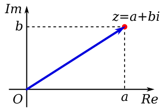
In mathematics, a complex number is an element of a number system that extends the real numbers with a specific element denoted i, called the imaginary unit and satisfying the equation ; every complex number can be expressed in the form , where a and b are real numbers. Because no real number satisfies the above equation, i was called an imaginary number by René Descartes. For the complex number , a is called the real part, and b is called the imaginary part. The set of complex numbers is denoted by either of the symbols or C. Despite the historical nomenclature "imaginary", complex numbers are regarded in the mathematical sciences as just as "real" as the real numbers and are fundamental in many aspects of the scientific description of the natural world.

<span class="mw-page-title-main">Ellipse</span> Plane curve: conic section

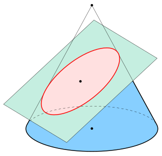
In mathematics, an ellipse is a plane curve surrounding two focal points, such that for all points on the curve, the sum of the two distances to the focal points is a constant. It generalizes a circle, which is the special type of ellipse in which the two focal points are the same. The elongation of an ellipse is measured by its eccentricity , a number ranging from to .

<span class="mw-page-title-main">Partial differential equation</span> Type of differential equation

In mathematics, a partial differential equation (PDE) is an equation which imposes relations between the various partial derivatives of a multivariable function.

In linear algebra, two vectors in an inner product space are orthonormal if they are orthogonal unit vectors. A set of vectors form an orthonormal set if all vectors in the set are mutually orthogonal and all of unit length. An orthonormal set which forms a basis is called an orthonormal basis.

<span class="mw-page-title-main">Multiplicative inverse</span> Number which when multiplied by x equals 1

In mathematics, a multiplicative inverse or reciprocal for a number x, denoted by 1/x or x−1, is a number which when multiplied by x yields the multiplicative identity, 1. The multiplicative inverse of a fraction a/b is b/a. For the multiplicative inverse of a real number, divide 1 by the number. For example, the reciprocal of 5 is one fifth (1/5 or 0.2), and the reciprocal of 0.25 is 1 divided by 0.25, or 4. The reciprocal function, the function f(x) that maps x to 1/x, is one of the simplest examples of a function which is its own inverse (an involution).

In signal processing, a finite impulse response (FIR) filter is a filter whose impulse response is of finite duration, because it settles to zero in finite time. This is in contrast to infinite impulse response (IIR) filters, which may have internal feedback and may continue to respond indefinitely.

<span class="mw-page-title-main">Buckling</span> Sudden change in shape of a structural component under load

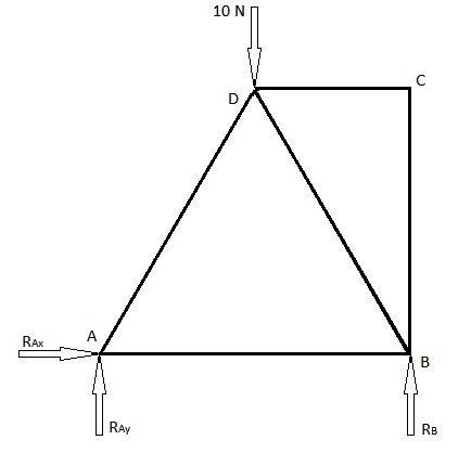
In structural engineering, buckling is the sudden change in shape (deformation) of a structural component under load, such as the bowing of a column under compression or the wrinkling of a plate under shear. If a structure is subjected to a gradually increasing load, when the load reaches a critical level, a member may suddenly change shape and the structure and component is said to have buckled. Euler's critical load and Johnson's parabolic formula are used to determine the buckling stress in slender columns.

In orbital mechanics, the eccentric anomaly is an angular parameter that defines the position of a body that is moving along an elliptic Kepler orbit. The eccentric anomaly is one of three angular parameters ("anomalies") that define a position along an orbit, the other two being the true anomaly and the mean anomaly.

<span class="mw-page-title-main">Arc length</span> Distance along a curve

Arc length is the distance between two points along a section of a curve.

<span class="mw-page-title-main">Euler–Bernoulli beam theory</span>

Euler–Bernoulli beam theory is a simplification of the linear theory of elasticity which provides a means of calculating the load-carrying and deflection characteristics of beams. It covers the case corresponding to small deflections of a beam that is subjected to lateral loads only. By ignoring the effects of shear deformation and rotatory inertia, it is thus a special case of Timoshenko–Ehrenfest beam theory. It was first enunciated circa 1750, but was not applied on a large scale until the development of the Eiffel Tower and the Ferris wheel in the late 19th century. Following these successful demonstrations, it quickly became a cornerstone of engineering and an enabler of the Second Industrial Revolution.

As one of the methods of structural analysis, the direct stiffness method, also known as the matrix stiffness method, is particularly suited for computer-automated analysis of complex structures including the statically indeterminate type. It is a matrix method that makes use of the members' stiffness relations for computing member forces and displacements in structures. The direct stiffness method is the most common implementation of the finite element method (FEM). In applying the method, the system must be modeled as a set of simpler, idealized elements interconnected at the nodes. The material stiffness properties of these elements are then, through matrix mathematics, compiled into a single matrix equation which governs the behaviour of the entire idealized structure. The structure’s unknown displacements and forces can then be determined by solving this equation. The direct stiffness method forms the basis for most commercial and free source finite element software.

The finite element method (FEM) is a powerful technique originally developed for numerical solution of complex problems in structural mechanics, and it remains the method of choice for complex systems. In the FEM, the structural system is modeled by a set of appropriate finite elements interconnected at discrete points called nodes. Elements may have physical properties such as thickness, coefficient of thermal expansion, density, Young's modulus, shear modulus and Poisson's ratio.

Structural dynamics is a type of structural analysis which covers the behavior of a structure subjected to dynamic loading. Dynamic loads include people, wind, waves, traffic, earthquakes, and blasts. Any structure can be subjected to dynamic loading. Dynamic analysis can be used to find dynamic displacements, time history, and modal analysis.

<span class="mw-page-title-main">Pendulum (mechanics)</span> Free swinging suspended body

A pendulum is a body suspended from a fixed support so that it swings freely back and forth under the influence of gravity. When a pendulum is displaced sideways from its resting, equilibrium position, it is subject to a restoring force due to gravity that will accelerate it back toward the equilibrium position. When released, the restoring force acting on the pendulum's mass causes it to oscillate about the equilibrium position, swinging it back and forth. The mathematics of pendulums are in general quite complicated. Simplifying assumptions can be made, which in the case of a simple pendulum allow the equations of motion to be solved analytically for small-angle oscillations.

<span class="mw-page-title-main">Contact mechanics</span> Study of the deformation of solids that touch each other

Contact mechanics is the study of the deformation of solids that touch each other at one or more points. A central distinction in contact mechanics is between stresses acting perpendicular to the contacting bodies' surfaces and frictional stresses acting tangentially between the surfaces. Normal contact mechanics or frictionless contact mechanics focuses on normal stresses caused by applied normal forces and by the adhesion present on surfaces in close contact, even if they are clean and dry. Frictional contact mechanics emphasizes the effect of friction forces.

<span class="mw-page-title-main">Deflection (engineering)</span> Degree to which part of a structural element is displaced under a given load

In structural engineering, deflection is the degree to which a part of a structural element is displaced under a load. It may refer to an angle or a distance.

In fracture mechanics, the energy release rate, , is the rate at which energy is transformed as a material undergoes fracture. Mathematically, the energy release rate is expressed as the decrease in total potential energy per increase in fracture surface area, and is thus expressed in terms of energy per unit area. Various energy balances can be constructed relating the energy released during fracture to the energy of the resulting new surface, as well as other dissipative processes such as plasticity and heat generation. The energy release rate is central to the field of fracture mechanics when solving problems and estimating material properties related to fracture and fatigue.

<span class="mw-page-title-main">Interval finite element</span>

In numerical analysis, the interval finite element method is a finite element method that uses interval parameters. Interval FEM can be applied in situations where it is not possible to get reliable probabilistic characteristics of the structure. This is important in concrete structures, wood structures, geomechanics, composite structures, biomechanics and in many other areas. The goal of the Interval Finite Element is to find upper and lower bounds of different characteristics of the model and use these results in the design process. This is so called worst case design, which is closely related to the limit state design.

<span class="mw-page-title-main">Structural engineering theory</span>

Structural engineering depends upon a detailed knowledge of loads, physics and materials to understand and predict how structures support and resist self-weight and imposed loads. To apply the knowledge successfully structural engineers will need a detailed knowledge of mathematics and of relevant empirical and theoretical design codes. They will also need to know about the corrosion resistance of the materials and structures, especially when those structures are exposed to the external environment.

Structural acoustics is the study of the mechanical waves in structures and how they interact with and radiate into adjacent media. The field of structural acoustics is often referred to as vibroacoustics in Europe and Asia. People that work in the field of structural acoustics are known as structural acousticians. The field of structural acoustics can be closely related to a number of other fields of acoustics including noise, transduction, underwater acoustics, and physical acoustics.

References