Types of mesh

Last updated

A mesh is a representation of a larger geometric domain by smaller discrete cells. Meshes are commonly used to compute solutions of partial differential equations and render computer graphics, and to analyze geographical and cartographic data. A mesh partitions space into elements (or cells or zones) over which the equations can be solved, which then approximates the solution over the larger domain. Element boundaries may be constrained to lie on internal or external boundaries within a model. Higher-quality (better-shaped) elements have better numerical properties, where what constitutes a "better" element depends on the general governing equations and the particular solution to the model instance.

Contents

Common cell shapes

Two-dimensional

Basic two-dimensional Cell shapes Two Dim Grid.PNG
Basic two-dimensional Cell shapes

There are two types of two-dimensional cell shapes that are commonly used. These are the triangle and the quadrilateral.

Computationally poor elements will have sharp internal angles or short edges or both.

Triangle

This cell shape consists of 3 sides and is one of the simplest types of mesh. A triangular surface mesh is always quick and easy to create. It is most common in unstructured grids.

Quadrilateral

This cell shape is a basic 4 sided one as shown in the figure. It is most common in structured grids.

Quadrilateral elements are usually excluded from being or becoming concave.

Three-dimensional

Basic three-dimensional cell shapes Three Dim Grid.PNG
Basic three-dimensional cell shapes

The basic 3-dimensional element are the tetrahedron, quadrilateral pyramid, triangular prism, and hexahedron. They all have triangular and quadrilateral faces.

Extruded 2-dimensional models may be represented entirely by the prisms and hexahedra as extruded triangles and quadrilaterals.

In general, quadrilateral faces in 3-dimensions may not be perfectly planar. A nonplanar quadrilateral face can be considered a thin tetrahedral volume that is shared by two neighboring elements.

Tetrahedron

A tetrahedron has 4 vertices, 6 edges, and is bounded by 4 triangular faces. In most cases a tetrahedral volume mesh can be generated automatically.

Pyramid

A quadrilaterally-based pyramid has 5 vertices, 8 edges, bounded by 4 triangular and 1 quadrilateral face. These are effectively used as transition elements between square and triangular faced elements and other in hybrid meshes and grids.

Triangular prism

A triangular prism has 6 vertices, 9 edges, bounded by 2 triangular and 3 quadrilateral faces. The advantage with this type of layer is that it resolves boundary layer efficiently.

Hexahedron

A hexahedron, a topological cube, has 8 vertices, 12 edges, bounded by 6 quadrilateral faces. It is also called a hex or a brick. [1] For the same cell amount, the accuracy of solutions in hexahedral meshes is the highest.

The pyramid and triangular prism zones can be considered computationally as degenerate hexahedrons, where some edges have been reduced to zero. Other degenerate forms of a hexahedron may also be represented.

Advanced Cells (Polyhedron)

A polyhedron (dual) element has any number of vertices, edges and faces. It usually requires more computing operations per cell due to the number of neighbours (typically 10). [2] Though this is made up for in the accuracy of the calculation.

Classification of grids

Structured grid Curvilinear grid.svg
Structured grid
Unstructured grid Example of 2D mesh.png
Unstructured grid

Structured grids

Structured grids are identified by regular connectivity. The possible element choices are quadrilateral in 2D and hexahedra in 3D. This model is highly space efficient, since the neighbourhood relationships are defined by storage arrangement. Some other advantages of structured grid over unstructured are better convergence and higher resolution. [3] [4] [5]

Unstructured grids

An unstructured grid is identified by irregular connectivity. It cannot easily be expressed as a two-dimensional or three-dimensional array in computer memory. This allows for any possible element that a solver might be able to use. Compared to structured meshes, for which the neighborhood relationships are implicit, this model can be highly space inefficient since it calls for explicit storage of neighborhood relationships. The storage requirements of a structured grid and of an unstructured grid are within a constant factor. These grids typically employ triangles in 2D and tetrahedral in 3D. [6]

Hybrid grids

A hybrid grid contains a mixture of structured portions and unstructured portions. It integrates the structured meshes and the unstructured meshes in an efficient manner. Those parts of the geometry that are regular can have structured grids and those that are complex can have unstructured grids. These grids can be non-conformal which means that grid lines don’t need to match at block boundaries. [7]

Mesh quality

A mesh is considered to have higher quality if a more accurate solution is calculated more quickly. Accuracy and speed are in tension. Decreasing the mesh size always increases the accuracy but also increases computational cost.

Accuracy depends on both discretization error and solution error. For discretization error, a given mesh is a discrete approximation of the space, and so can only provide an approximate solution, even when equations are solved exactly. (In computer graphics ray tracing, the number of rays fired is another source of discretization error.) For solution error, for PDEs many iterations over the entire mesh are required. The calculation is terminated early, before the equations are solved exactly. The choice of mesh element type affects both discretization and solution error.

Accuracy depends on both the total number of elements, and the shape of individual elements. The speed of each iteration grows (linearly) with the number of elements, and the number of iterations needed depends on the local solution value and gradient compared to the shape and size of local elements.

Solution precision

A coarse mesh may provide an accurate solution if the solution is a constant, so the precision depends on the particular problem instance. One can selectively refine the mesh in areas where the solution gradients are high, thus increasing fidelity there. Accuracy, including interpolated values within an element, depends on the element type and shape.

Rate of convergence

Each iteration reduces the error between the calculated and true solution. A faster rate of convergence means smaller error with fewer iterations.

A mesh of inferior quality may leave out important features such as the boundary layer for fluid flow. The discretization error will be large and the rate of convergence will be impaired; the solution may not converge at all.

Grid independence

A solution is considered grid-independent if the discretization and solution error are small enough given sufficient iterations. This is essential to know for comparative results. A mesh convergence study consists of refining elements and comparing the refined solutions to the coarse solutions. If further refinement (or other changes) does not significantly change the solution, the mesh is an "Independent Grid."

Deciding the type of mesh

Skewness based on equilateral volume Skweness.PNG
Skewness based on equilateral volume

If the accuracy is of the highest concern then hexahedral mesh is the most preferable one. The density of the mesh is required to be sufficiently high in order to capture all the flow features but on the same note, it should not be so high that it captures unnecessary details of the flow, thus burdening the CPU and wasting more time. Whenever a wall is present, the mesh adjacent to the wall is fine enough to resolve the boundary layer flow and generally quad, hex and prism cells are preferred over triangles, tetrahedrons and pyramids. Quad and Hex cells can be stretched where the flow is fully developed and one-dimensional.

Depicts the skewness of a quadrilateral Skewnessquad.PNG
Depicts the skewness of a quadrilateral

Based on the skewness, smoothness, and aspect ratio, the suitability of the mesh can be decided. [8]

Skewness

The skewness of a grid is an apt indicator of the mesh quality and suitability. Large skewness compromises the accuracy of the interpolated regions. There are three methods of determining the skewness of a grid.

Based on equilateral volume

This method is applicable to triangles and tetrahedral only and is the default method.

Smooth and large jump change Smooth and Large Jump.PNG
Smooth and large jump change

Based on the deviation from normalized equilateral angle

This method applies to all cell and face shapes and is almost always used for prisms and pyramids

Equiangular skew

Another common measure of quality is based on equiangular skew.

where:

  • is the largest angle in a face or cell,
  • is the smallest angle in a face or cell,
  • is the angle for equi-angular face or cell i.e. 60 for a triangle and 90 for a square.

A skewness' of 0 is the best possible one and a skewness of one is almost never preferred. For Hex and quad cells, skewness should not exceed 0.85 to obtain a fairly accurate solution.

Depicts the changes in aspect ratio Aspect ratio grid.PNG
Depicts the changes in aspect ratio

For triangular cells, skewness should not exceed 0.85 and for quadrilateral cells, skewness should not exceed 0.9.

Smoothness

The change in size should also be smooth. There should not be sudden jumps in the size of the cell because this may cause erroneous results at nearby nodes.

Aspect ratio

It is the ratio of longest to the shortest side in a cell. Ideally it should be equal to 1 to ensure best results. For multidimensional flow, it should be near to one. Also local variations in cell size should be minimal, i.e. adjacent cell sizes should not vary by more than 20%. Having a large aspect ratio can result in an interpolation error of unacceptable magnitude.

Mesh generation and improvement

See also mesh generation and principles of grid generation. In two dimensions, flipping and smoothing are powerful tools for adapting a poor mesh into a good mesh. Flipping involves combining two triangles to form a quadrilateral, then splitting the quadrilateral in the other direction to produce two new triangles. Flipping is used to improve quality measures of a triangle such as skewness. Mesh smoothing enhances element shapes and overall mesh quality by adjusting the location of mesh vertices. In mesh smoothing, core features such as non-zero pattern of the linear system are preserved as the topology of the mesh remains invariant. Laplacian smoothing is the most commonly used smoothing technique.

See also

Related Research Articles

In geometry, a polygon is a plane figure made up of line segments connected to form a closed polygonal chain.

<span class="mw-page-title-main">Triangular bipyramid</span> Two tetrahedra joined along one face

In geometry, the triangular bipyramid is the hexahedron with six triangular faces, constructed by attaching two tetrahedrons face-to-face. The same shape is also called the triangular dipyramid or trigonal bipyramid. If these tetrahedrons are regular, all faces of triangular bipyramid are equilateral. It is an example of a deltahedron and of a Johnson solid.

<span class="mw-page-title-main">Triaugmented triangular prism</span> Convex polyhedron with 14 triangle faces

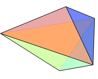
The triaugmented triangular prism, in geometry, is a convex polyhedron with 14 equilateral triangles as its faces. It can be constructed from a triangular prism by attaching equilateral square pyramids to each of its three square faces. The same shape is also called the tetrakis triangular prism, tricapped trigonal prism, tetracaidecadeltahedron, or tetrakaidecadeltahedron; these last names mean a polyhedron with 14 triangular faces. It is an example of a deltahedron and of a Johnson solid.

<span class="mw-page-title-main">Polygonal modeling</span> Object modeling method

In 3D computer graphics, polygonal modeling is an approach for modeling objects by representing or approximating their surfaces using polygon meshes. Polygonal modeling is well suited to scanline rendering and is therefore the method of choice for real-time computer graphics. Alternate methods of representing 3D objects include NURBS surfaces, subdivision surfaces, and equation-based representations used in ray tracers.

<span class="mw-page-title-main">Duoprism</span> Cartesian product of two polytopes

In geometry of 4 dimensions or higher, a double prism or duoprism is a polytope resulting from the Cartesian product of two polytopes, each of two dimensions or higher. The Cartesian product of an n-polytope and an m-polytope is an (n+m)-polytope, where n and m are dimensions of 2 (polygon) or higher.

<span class="mw-page-title-main">Lloyd's algorithm</span> Algorithm used for points in euclidean space

In electrical engineering and computer science, Lloyd's algorithm, also known as Voronoi iteration or relaxation, is an algorithm named after Stuart P. Lloyd for finding evenly spaced sets of points in subsets of Euclidean spaces and partitions of these subsets into well-shaped and uniformly sized convex cells. Like the closely related k-means clustering algorithm, it repeatedly finds the centroid of each set in the partition and then re-partitions the input according to which of these centroids is closest. In this setting, the mean operation is an integral over a region of space, and the nearest centroid operation results in Voronoi diagrams.

<span class="mw-page-title-main">Rhombohedron</span> Polyhedron with six rhombi as faces

In geometry, a rhombohedron is a three-dimensional figure with six faces which are rhombi. It is a special case of a parallelepiped where all edges are the same length. It can be used to define the rhombohedral lattice system, a honeycomb with rhombohedral cells. A cube is a special case of a rhombohedron with all sides square.

<span class="mw-page-title-main">Triangular prism</span> Prism with a 3-sided base

In geometry, a triangular prism or trigonal prism is a prism with 2 triangular bases. If the edges pair with each triangle's vertex and if they are perpendicular to the base, it is a right triangular prism. A right triangular prism may be both semiregular and uniform.

<span class="mw-page-title-main">Mesh generation</span> Subdivision of space into cells

Mesh generation is the practice of creating a mesh, a subdivision of a continuous geometric space into discrete geometric and topological cells. Often these cells form a simplicial complex. Usually the cells partition the geometric input domain. Mesh cells are used as discrete local approximations of the larger domain. Meshes are created by computer algorithms, often with human guidance through a GUI, depending on the complexity of the domain and the type of mesh desired. A typical goal is to create a mesh that accurately captures the input domain geometry, with high-quality (well-shaped) cells, and without so many cells as to make subsequent calculations intractable. The mesh should also be fine in areas that are important for the subsequent calculations.

<span class="mw-page-title-main">Regular grid</span> Tessellation of n-dimensional Euclidean space by congruent parallelotopes

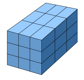
A regular grid is a tessellation of n-dimensional Euclidean space by congruent parallelotopes. Its opposite is irregular grid.

<span class="mw-page-title-main">Unstructured grid</span> Unstructured (or irregular) grid is a tessellation of a part of the Euclidean plane

An unstructured grid or irregular grid is a tessellation of a part of the Euclidean plane or Euclidean space by simple shapes, such as triangles or tetrahedra, in an irregular pattern. Grids of this type may be used in finite element analysis when the input to be analyzed has an irregular shape.

<span class="mw-page-title-main">Finite element method</span> Numerical method for solving physical or engineering problems

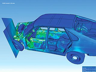
The finite element method (FEM) is a popular method for numerically solving differential equations arising in engineering and mathematical modeling. Typical problem areas of interest include the traditional fields of structural analysis, heat transfer, fluid flow, mass transport, and electromagnetic potential.

hp-FEM is a generalization of the finite element method (FEM) for solving partial differential equations numerically based on piecewise-polynomial approximations. hp-FEM originates from the discovery by Barna A. Szabó and Ivo Babuška that the finite element method converges exponentially fast when the mesh is refined using a suitable combination of h-refinements and p-refinements .The exponential convergence of hp-FEM has been observed by numerous independent researchers.

Grid or mesh is defined as smaller shapes formed after discretisation of geometric domain. Mesh or grid can be in 3- dimension and 2-dimension. Meshing has applications in the fields of geography, designing, computational fluid dynamics. and many more places. The two-dimensional meshing includes simple polygon, polygon with holes, multiple domain and curved domain. In three dimensions there are three types of inputs. They are simple polyhedron, geometrical polyhedron and multiple polyhedrons. Before defining the mesh type it is necessary to understand elements.

In graph drawing and geometric graph theory, a Tutte embedding or barycentric embedding of a simple, 3-vertex-connected, planar graph is a crossing-free straight-line embedding with the properties that the outer face is a convex polygon and that each interior vertex is at the average of its neighbors' positions. If the outer polygon is fixed, this condition on the interior vertices determines their position uniquely as the solution to a system of linear equations. Solving the equations geometrically produces a planar embedding. Tutte's spring theorem, proven by W. T. Tutte, states that this unique solution is always crossing-free, and more strongly that every face of the resulting planar embedding is convex. It is called the spring theorem because such an embedding can be found as the equilibrium position for a system of springs representing the edges of the graph.

<span class="mw-page-title-main">3-3 duoprism</span>

In the geometry of 4 dimensions, the 3-3 duoprism or triangular duoprism is a four-dimensional convex polytope. It can be constructed as the Cartesian product of two triangles and is the simplest of an infinite family of four-dimensional polytopes constructed as Cartesian products of two polygons, the duoprisms.

<span class="mw-page-title-main">Ten-of-diamonds decahedron</span>

In geometry, the ten-of-diamonds decahedron is a space-filling polyhedron with 10 faces, 2 opposite rhombi with orthogonal major axes, connected by 8 identical isosceles triangle faces. Although it is convex, it is not a Johnson solid because its faces are not composed entirely of regular polygons. Michael Goldberg named it after a playing card, as a 10-faced polyhedron with two opposite rhombic (diamond-shaped) faces. He catalogued it in a 1982 paper as 10-II, the second in a list of 26 known space-filling decahedra.

JMesh is a JSON-based portable and extensible file format for the storage and interchange of unstructured geometric data, including discretized geometries such as triangular and tetrahedral meshes, parametric geometries such as NURBS curves and surfaces, and constructive geometries such as constructive solid geometry (CGS) of shape primitives and meshes. Built upon the JData specification, a JMesh file utilizes the JSON and Universal Binary JSON (UBJSON) constructs to serialize and encode geometric data structures, therefore, it can be directly processed by most existing JSON and UBJSON parsers. The JMesh specification defines a list of JSON-compatible constructs to encode geometric data, including N-dimensional (ND) vertices, curves, surfaces, solid elements, shape primitives, their interactions and spatial relations, together with their associated properties, such as numerical values, colors, normals, materials, textures and other properties related to graphics data manipulation, 3-D fabrication, computer graphics rendering and animations.

References

  1. "Hexahedron elements" (PDF). Archived from the original (PDF) on 2015-02-24. Retrieved 2015-04-13.
  2. "Archived copy" (PDF). Archived from the original (PDF) on 2013-12-06. Retrieved 2018-01-10.{{cite web}}: CS1 maint: archived copy as title (link)
  3. "Quality and Control - Two Reasons Why Structured Grids Aren't Going Away".
  4. Castillo, J.E. (1991), "Mathematical aspects of grid Generation", Society for Industrial and Applied Mathematics, Philadelphia
  5. George, P.L. (1991), Automatic Mesh Generation
  6. Mavriplis, D.J. (1996), "Mesh Generation and adaptivity for complex geometries and flows", Handbook of Computational Fluid Mechanics
  7. Bern, Marshall; Plassmann, Paul (2000), "Mesh Generation", Handbook of Computational Geometry. Elsevier Science
  8. "Meshing, Lecture 7". Andre Bakker. Retrieved 2012-11-10.