Production set

Last updated March 12, 2024

In economics the production set is a construct representing the possible inputs and outputs to a production process.

If the commodities in the economy are (labour, corn, flour, bread) and a mill uses one unit of labour to produce 8 units of flour from 10 units of corn, then its production vector is (–1,–10,8,0). If it needs the same amount of labour to run at half capacity then the production vector (–1,–5,4,0) would also be operationally possible. The set of all operationally possible production vectors is the mill's production set.

If y is a production vector and p is the economy's price vector, then p·y is the value of net output. The mill's owner will normally choose y from the production set to maximise this quantity. p·y is defined as the 'profit' of the vector y, and the mill-owner's behaviour is described as 'profit-maximising'.^[1]

Properties of production sets

The following properties may be predicated of production sets.^[2]

Non-emptiness. The producer has at least one possible course of action. Always holds.
Closure. The production set includes its own boundary. This is a technical property which always holds in practice.
Separability. A production set is separable into inputs and outputs if every field is either non-negative in all elements or non-positive in all elements. This normally holds for individual enterprises but not, for instance, for a national economy.
No free lunch. It is impossible to produce something from nothing. Mathematically there is no vector in the production set with at least one positive entry and no negative entries. Always holds.
Possibility of inaction. The zero vector belongs to the production set; in other words, it is possible to produce nothing by consuming nothing. This property almost never holds exactly: resources will be needed either to wind up a concern or to maintain it while dormant. The property may be a useful approximation.
Free disposal. If y is an element of production set Y, then so is any vector which consumes more of a given input or produces less of a given output. Mathematically, if e is a vector none of whose entries is negative, and if y ∈ Y, then y – e ∈ Y. This too may be a useful approximation.
Single output. Production is often based on units (e.g. flour mills) which produce a single output from more than one input. A separable production set has a single output if exactly one field contains a positive entry.
Labour consumption. Labour is usually an input to all elements of a production set which have any positive output.
Irreversibility . If y ∈ Y and y≠0 then (–y) ∉ Y. Always holds in practice.
Convexity. If two vectors lie within the production set, then so do all intermediate points. This often holds as an approximation but cannot apply exactly if inputs or outputs comprise discrete units.
Additivity (or free entry ). This property is relevant to the production set of an industry or of an economy but not for instance to a single flour mill. It means that if production vector y is possible, and so is y', then so too is y+y'. So if a mill can be built with a view to running in one way, and another mill can be built with a view to running in another way, then both can be built to produce the sum of intended outputs from the sum of intended inputs. Free entry is a postulate of perfect competition.
Returns to scale and economies of scale . See below.

The production function

If a production set is separable and has a single output, then a function F(y) can be constructed whose value is the maximum quantity of output obtainable for given inputs, and whose domain is the set of input subvectors represented in the production set. This is known as the production function.

If a production set is separable then we may define a "production value function" f_p(x) in terms of a price vector p. If x is a monetary quantity, then f_p(x) is the maximum monetary value of output obtainable in Y from inputs whose cost is x.

Returns to scale

Constant returns to scale mean that if y is in the production set, then so too is λy for any positive λ. Returns might be constant over a region; for instance, so long as λ is not too far from 1 for a given y. There is no entirely satisfactory way to define increasing or decreasing returns to scale for general production sets.

If the production set Y can be represented by a production function F whose argument is the input subvector of a production vector, then increasing returns to scale are available if F(λy) > λF(y) for all λ > 1 and F(λy) < λF(y) for all λ<1. A converse condition can be stated for decreasing returns to scale.

Economies of scale

If Y is a separable production set with a production value function f_p, then (positive) economies of scale are present if f_p(λx) > λf_p(x) for all λ > 1 and f_p(λx) < λf_p(x) for all λ < 1. The opposite condition may be referred to as negative economies (or diseconomies) of scale.

If Y has a single output and prices are positive, then positive economies of scale are equivalent to increasing returns to scale.

As with returns to scale, economies of scale may apply over a region. If a mill is operating below capacity then it will offer positive economies of scale, but as it approaches capacity the economies will become negative. Economies of scale for the firm are important in influencing an industry's tendency to concentrate in the direction of monopoly or disaggregate in the direction of perfect competition.

Limitation

The components of a production vector are conventionally portrayed as flows (see Stock and flow), whereas more general treatments regard production as combining stocks (e.g. land) and flows (e.g. labour) (see Factors of production). Accordingly, the simple definition of 'profit' as the net value of output does not correspond to its meaning elsewhere in economics (see Profit (economics)).

Related Research Articles

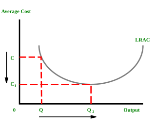
In microeconomics, economies of scale are the cost advantages that enterprises obtain due to their scale of operation, and are typically measured by the amount of output produced per unit of time. A decrease in cost per unit of output enables an increase in scale. At the basis of economies of scale, there may be technical, statistical, organizational or related factors to the degree of market control.

Physical capital represents in economics one of the three primary factors of production. Physical capital is the apparatus used to produce a good and services. Physical capital represents the tangible man-made goods that help and support the production. Inventory, cash, equipment or real estate are all examples of physical capital.

In machine learning, the perceptron is an algorithm for supervised learning of binary classifiers. A binary classifier is a function which can decide whether or not an input, represented by a vector of numbers, belongs to some specific class. It is a type of linear classifier, i.e. a classification algorithm that makes its predictions based on a linear predictor function combining a set of weights with the feature vector.

In economics, the marginal cost is the change in the total cost that arises when the quantity produced is increased, i.e. the cost of producing additional quantity. In some contexts, it refers to an increment of one unit of output, and in others it refers to the rate of change of total cost as output is increased by an infinitesimal amount. As Figure 1 shows, the marginal cost is measured in dollars per unit, whereas total cost is in dollars, and the marginal cost is the slope of the total cost, the rate at which it increases with output. Marginal cost is different from average cost, which is the total cost divided by the number of units produced.

<span class="mw-page-title-main">Cobb–Douglas production function</span> Macroeconomic formula that describes productivity

In economics and econometrics, the Cobb–Douglas production function is a particular functional form of the production function, widely used to represent the technological relationship between the amounts of two or more inputs and the amount of output that can be produced by those inputs. The Cobb–Douglas form was developed and tested against statistical evidence by Charles Cobb and Paul Douglas between 1927 and 1947; according to Douglas, the functional form itself was developed earlier by Philip Wicksteed.

In mathematics, the Hessian matrix, Hessian or Hesse matrix is a square matrix of second-order partial derivatives of a scalar-valued function, or scalar field. It describes the local curvature of a function of many variables. The Hessian matrix was developed in the 19th century by the German mathematician Ludwig Otto Hesse and later named after him. Hesse originally used the term "functional determinants". The Hessian is sometimes denoted by H or, ambiguously, by ∇².

In economics, a production function gives the technological relation between quantities of physical inputs and quantities of output of goods. The production function is one of the key concepts of mainstream neoclassical theories, used to define marginal product and to distinguish allocative efficiency, a key focus of economics. One important purpose of the production function is to address allocative efficiency in the use of factor inputs in production and the resulting distribution of income to those factors, while abstracting away from the technological problems of achieving technical efficiency, as an engineer or professional manager might understand it.

<span class="mw-page-title-main">Conditional (computer programming)</span> Control flow statement that executes code according to some condition(s)

In computer science, conditionals are programming language commands for handling decisions. Specifically, conditionals perform different computations or actions depending on whether a programmer-defined Boolean condition evaluates to true or false. In terms of control flow, the decision is always achieved by selectively altering the control flow based on some condition . Although dynamic dispatch is not usually classified as a conditional construct, it is another way to select between alternatives at runtime. Conditional statements are the checkpoints in the programme that determines behaviour according to situation.

In economics, average cost (AC) or unit cost is equal to total cost (TC) divided by the number of units of a good produced :

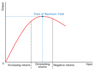
In economics, diminishing returns are the decrease in marginal (incremental) output of a production process as the amount of a single factor of production is incrementally increased, holding all other factors of production equal. The law of diminishing returns states that in productive processes, increasing a factor of production by one unit, while holding all other production factors constant, will at some point return a lower unit of output per incremental unit of input. The law of diminishing returns does not cause a decrease in overall production capabilities, rather it defines a point on a production curve whereby producing an additional unit of output will result in a loss and is known as negative returns. Under diminishing returns, output remains positive, but productivity and efficiency decrease.

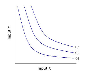
<span class="mw-page-title-main">Isoquant</span> Contour line in microeconomics

An isoquant, in microeconomics, is a contour line drawn through the set of points at which the same quantity of output is produced while changing the quantities of two or more inputs. The x and y axis on an isoquant represent two relevant inputs, which are usually a factor of production such as labour, capital, land, or organisation. An isoquant may also be known as an “Iso-Product Curve”, or an “Equal Product Curve”.

In economics, an input–output model is a quantitative economic model that represents the interdependencies between different sectors of a national economy or different regional economies. Wassily Leontief (1906–1999) is credited with developing this type of analysis and earned the Nobel Prize in Economics for his development of this model.

In matrix theory, the Perron–Frobenius theorem, proved by Oskar Perron and Georg Frobenius, asserts that a real square matrix with positive entries has a unique eigenvalue of largest magnitude and that eigenvalue is real. The corresponding eigenvector can be chosen to have strictly positive components, and also asserts a similar statement for certain classes of nonnegative matrices. This theorem has important applications to probability theory ; to the theory of dynamical systems ; to economics ; to demography ; to social networks ; to Internet search engines (PageRank); and even to ranking of American football teams. The first to discuss the ordering of players within tournaments using Perron–Frobenius eigenvectors is Edmund Landau.

In economics, a cost curve is a graph of the costs of production as a function of total quantity produced. In a free market economy, productively efficient firms optimize their production process by minimizing cost consistent with each possible level of production, and the result is a cost curve. Profit-maximizing firms use cost curves to decide output quantities. There are various types of cost curves, all related to each other, including total and average cost curves; marginal cost curves, which are equal to the differential of the total cost curves; and variable cost curves. Some are applicable to the short run, others to the long run.

In mathematics, an operation is a function which takes zero or more input values to a well-defined output value. The number of operands is the arity of the operation.

In statistics, data transformation is the application of a deterministic mathematical function to each point in a data set—that is, each data point z_i is replaced with the transformed value y_i = f(z_i), where f is a function. Transforms are usually applied so that the data appear to more closely meet the assumptions of a statistical inference procedure that is to be applied, or to improve the interpretability or appearance of graphs.

Production is the process of combining various inputs, both material and immaterial in order to create output. Ideally this output will be a good or service which has value and contributes to the utility of individuals. The area of economics that focuses on production is called production theory, and it is closely related to the consumption theory of economics.

In economics, the marginal product of labor (MP_L) is the change in output that results from employing an added unit of labor. It is a feature of the production function and depends on the amounts of physical capital and labor already in use.

Kernel methods are a well-established tool to analyze the relationship between input data and the corresponding output of a function. Kernels encapsulate the properties of functions in a computationally efficient way and allow algorithms to easily swap functions of varying complexity.

Environmentally extended input–output analysis (EEIOA) is used in environmental accounting as a tool which reflects production and consumption structures within one or several economies. As such, it is becoming an important addition to material flow accounting.

References

↑ Intermediate Microeconomics, Hal R. Varian 1999, W. W. Norton & Company; 5th edition
↑ Mas-Colell, Andreu; Whinston, Michael D.; Jerry R. Green (1995). Microeconomic Theory. New York: Oxford University Press. ISBN 0-19-507340-1.

This page is based on this Wikipedia article
Text is available under the CC BY-SA 4.0 license; additional terms may apply.
Images, videos and audio are available under their respective licenses.

[1] Intermediate Microeconomics, Hal R. Varian 1999, W. W. Norton & Company; 5th edition

[2] Mas-Colell, Andreu; Whinston, Michael D.; Jerry R. Green (1995). Microeconomic Theory. New York: Oxford University Press. ISBN 0-19-507340-1.

[1]

[2]

v t e Microeconomics
Major topics	Aggregation Budget set Consumer choice Convexity and non-convexity Cost Average Marginal Opportunity Implicit Social Sunk Transaction Cost–benefit analysis Deadweight loss Distribution Economies of scale Economies of scope Elasticity Cross elasticity of demand Price elasticity of demand Price elasticity of supply Equilibrium General Exchange Externality Firms Goods and services Goods Service Household Income–consumption curve Information Indifference curve Intertemporal choice Market Market failure Market structure Competition Monopolistic Perfect Duopoly Monopoly Bilateral Complementary Monopsony Oligopoly Oligopsony Pareto efficiency Preferences Price Price controls Price ceiling Price floor Price discrimination Price signal Price system/Free Production Profit Public goods Rationing Rent Returns to scale Risk aversion Scarcity Shortage/Excess supply Substitution effect Surplus Social choice Supply and demand Demand/Law of demand Supply/Law of supply Uncertainty Utility Expected Marginal Wage
Subfields	Behavioral Business Computational Statistical decision theory Econometrics Engineering economics Civil engineering economics Evolutionary Experimental Game theory Industrial organization Institutional Labor Law Managerial Mathematical Microfoundations of macroeconomics Operations research Optimization Welfare
See also	Economics Applied Macroeconomics Political economy
Category