Minimum bottleneck spanning tree

In mathematics, a minimum bottleneck spanning tree (MBST) in an undirected graph is a spanning tree in which the most expensive edge is as cheap as possible. A bottleneck edge is the highest weighted edge in a spanning tree. A spanning tree is a minimum bottleneck spanning tree if the graph does not contain a spanning tree with a smaller bottleneck edge weight. ^[1] For a directed graph, a similar problem is known as Minimum Bottleneck Spanning Arborescence (MBSA).

Definitions

Undirected graphs

Minimal Bottleneck Spanning Tree ⁠${\displaystyle G(V,E)}$⁠

In an undirected graph G(V, E) and a function w : E → R, let S be the set of all spanning trees T_i. Let B(T_i) be the maximum weight edge for any spanning tree T_i. We define subset of minimum bottleneck spanning trees S′ such that for every T_j ∈ S′ and T_k ∈ S we have B(T_j) ≤ B(T_k) for all i and k. ^[2]

The graph on the right is an example of MBST, the red edges in the graph form a MBST of G(V, E).

Directed graphs

Minimal Bottleneck Spanning Arborescence G(V,E)

An arborescence of graph G is a directed tree of G which contains a directed path from a specified node L to each node of a subset V′ of V \{L}. Node L is called the root of arborescence. An arborescence is a spanning arborescence if V′ = V \{L}. MBST in this case is a spanning arborescence with the minimum bottleneck edge. An MBST in this case is called a Minimum Bottleneck Spanning Arborescence (MBSA).

The graph on the right is an example of MBSA, the red edges in the graph form a MBSA of G(V, E).

Properties

A MST (or minimum spanning tree) is necessarily a MBST, but a MBST is not necessarily a MST. ^[3]

^[4]

Camerini's algorithm for undirected graphs

Camerini proposed ^[5] an algorithm used to obtain a minimum bottleneck spanning tree (MBST) in a given undirected, connected, edge-weighted graph in 1978. It half divides edges into two sets. The weights of edges in one set are no more than that in the other. If a spanning tree exists in subgraph composed solely with edges in smaller edges set, it then computes a MBST in the subgraph, a MBST of the subgraph is exactly a MBST of the original graph. If a spanning tree does not exist, it combines each disconnected component into a new super vertex, then computes a MBST in the graph formed by these super vertices and edges in the larger edges set. A forest in each disconnected component is part of a MBST in original graph. Repeat this process until two (super) vertices are left in the graph and a single edge with smallest weight between them is to be added. A MBST is found consisting of all the edges found in previous steps. ^[4]

Pseudocode

The procedure has two input parameters. G is a graph, w is a weights array of all edges in the graph G. ^[6]

function MBST(graph G, weights w)     E ← the set of edges of Gif | E | = 1 thenreturnEelseA ← half edges in E whose weights are no less than the median weight         B ← E - AF ← forest of GBifF is a spanning tree thenreturn MBST(GB,w)         elsereturn MBST((GA)η, w) ${\displaystyle \cup }$F

In the above (G_A)_η is the subgraph composed of super vertices (by regarding vertices in a disconnected component as one) and edges in A.

Running time

The algorithm is running in O (E) time, where E is the number of edges. This bound is achieved as follows:

• dividing into two sets with median-finding algorithms in O(E)
• finding a forest in O(E)
• considering half edges in E in each iteration T(E)=T(E/2)+O(E). By the Master theorem , the overall time complexity is O (E).

NOTE: The run time estimate O(E) instead of O(E+V) (traversing a graph takes O(E+V) time), but for this case the graph is connected, therefore V-1<=E, hence, O(E+V)=O(E).

Example

In the following example green edges are used to form a MBST and dashed red areas indicate super vertices formed during the algorithm steps.

	The algorithm half divides edges in two sets with respect to weights. Green edges are those edges whose weights are as small as possible.
	Since there is a spanning tree in the subgraph formed solely with edges in the smaller edges set. Repeat finding a MBST in this subgraph.
	Since there is not a spanning tree in current subgraph formed with edges in the current smaller edges set. Combine the vertices of a disconnected component to a super vertex (denoted by a dashed red area) and then find a MBST in the subgraph formed with super vertices and edges in larger edges set. A forest formed within each disconnected component will be part of a MBST in the original graph.
	Repeat similar steps by combining more vertices into a super vertex.
	The algorithm finally obtains a MBST by using edges it found during the algorithm.

MBSA algorithms for directed graphs

There are two algorithms available for directed graph: Camerini's algorithm for finding MBSA and another from Gabow and Tarjan. ^[4]

Camerini's algorithm for MBSA

For a directed graph, Camerini's algorithm focuses on finding the set of edges that would have its maximum cost as the bottleneck cost of the MBSA. This is done by partitioning the set of edges E into two sets A and B and maintaining the set T that is the set in which it is known that G_T does not have a spanning arborescence, increasing T by B whenever the maximal arborescence of G(B ∪ T) is not a spanning arborescence of G, otherwise we decrease E by A. The total time complexity is O(E log E). ^{[5] [4]}

Pseudocode

function MBSA(G, w, T) isE ← the set of edges of Gif | E − T | > 1 thenA ← UH(E-T)         B ← (E − T) − AF ← BUSH(GBUT)         ifF is a spanning arborescence of G then             S ← F             MBSA((GBUT), w, T)         else             MBSA(G, w, TUB);

1. T represents a subset of E for which it is known that G_T does not contain any spanning arborescence rooted at node “a”. Initially T is empty
2. UH takes (E−T) set of edges in G and returns A ⊂ (E−T) such that:
   1. ${\displaystyle |A|=\left\lfloor {\frac {(|E-T|)}{2}}\right\rfloor }$
   2. W_a≥ W_b , for a ∈ A and b ∈ B
3. BUSH(G) returns a maximal arborescence of G rooted at node “a”
4. The final result will be S

Example

	After running the first iteration of this algorithm, we get the F and F is not a spanning arborescence of G, So we run the code ⁠${\displaystyle MBSA(G,w,T\cup B).}$⁠
	In the second iteration, we get the ${\displaystyle F'}$ and ${\displaystyle F'}$ is also not a spanning arborescence of G, So we run the code ${\displaystyle MBSA(G,w,T'\cup B')}$
	In the third iteration, we get the ${\displaystyle F''}$ and ${\displaystyle F''}$ is a spanning arborescence of G, So we run the code ${\displaystyle MBSA(G_{T''\cup B''},w,T'')}$
	when we run the ${\displaystyle MBSA(G_{T''\cup B''},w,T'')}$, the ${\displaystyle |E-T|}$ is equal to 1, which is not larger than 1, so the algorithm return and the final result is ${\displaystyle S=F''}$.

Gabow and Tarjan algorithm for MBSA

Gabow and Tarjan provided a modification of Dijkstra's algorithm for single-source shortest path that produces an MBSA. Their algorithm runs in O(E + V log V) time if Fibonacci heap used. ^[7]

Pseudocode

 For a graph G(V,E), F is a collection of vertices in V.   Initially, F = {s} where s is the starting point of the graph G and c(s) = -∞   1  function MBSA-GT(G, w, T)  2      repeat |V| times  3          Select v with minimum c(v) from F;   4          Delete it from the F;  5          for∀ edge(v, w) do  6              ifw∉F or ∉ Tree then  7                  add w to F;            8                  c(w) = c(v,w);  9                  p(w) = v;       10             else  11                 ifw∈F and c(w) > c(v, w)then  12                     c(w) = c(v, w);  13                     p(w) = v;

Example

The following example shows that how the algorithm works.

At the first step of the algorithm, we select the root s from the graph G, in the above figure, vertex 6 is the root s. Then we found all the edge(6,w) ∈ E and their cost c(6,w), where w ∈ V.

Next we move to the vertex 5 in the graph G, we found all the edge(5,w) ∈ E and their cost c(5,w), where w ∈ V.

Next we move to the vertex 4 in the graph G, we found all the edge(4,w) ∈ E and their cost c(4,w), where w ∈ V. We find that the edge(4,5) > edge(6.5), so we keep edge(6,5) and remove the edge(4,5).

Next we move to the vertex 1 in the graph G, we found all the edge(1,w) ∈ E and their cost c(1,w), where w ∈ V. We find that the edge(5,2) > edge(1,2), so we remove edge(5,2) and keep the edge(1,2).

Next we move to the vertex 2 in the graph G, we found all the edge(2,w) ∈ E and their cost c(2,w), where w ∈ V.

Next we move to the vertex 3 in the graph G, we found all the edge(3,w) ∈ E and their cost c(3,w), where w ∈ V. We find that the edge(3,4) > edge(6,4), so we remove the edge(3,4) and keep the edge(6,4).

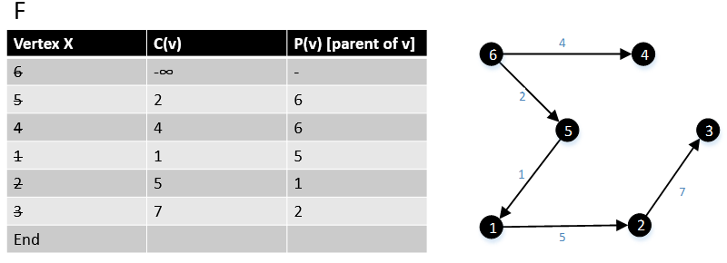
After we loop through all the vertices in the graph G, the algorithm has finished.

Another approach proposed by Tarjan and Gabow with bound of O(E log^* V) for sparse graphs, in which it is very similar to Camerini’s algorithm for MBSA, but rather than partitioning the set of edges into two sets per each iteration, K(i) was introduced in which i is the number of splits that has taken place or in other words the iteration number, and K(i) is an increasing function that denotes the number of partitioned sets that one should have per iteration. K(i) = 2^k(i − 1) with k(1) = 2. The algorithm finds λ^* in which it is the value of the bottleneck edge in any MBSA. After λ^* is found any spanning arborescence in G(λ^*) is an MBSA in which G(λ^*) is the graph where all its edge's costs are ≤ λ^*. ^{[4] [7]}

References

1. Everything about Bottleneck Spanning Tree
2. Murali, T. M. (2009), Applications of Minimum Spanning Trees (PDF)
3. in question 3 you have a proof for this claim (PDF)
4. Traboulsi, Ahmad (2014), Bottleneck Spanning Trees (PDF), archived from the original (PDF) on 2016-03-04, retrieved 2014-12-28
5. Camerini, P.M. (1978), "The min-max spanning tree problem and some extensions", Information Processing Letters , 7 (1): 10–14, doi:10.1016/0020-0190(78)90030-3
6. Cui, Yuxiang (2013), Minimum Bottleneck Spanning Tree (PDF), archived from the original (PDF) on 2016-03-04, retrieved 2014-12-28
7. Gabow, Harold N; Tarjan, Robert E (1988). "Algorithms for two bottleneck optimization problems". Journal of Algorithms. 9 (3): 411–417. doi:10.1016/0196-6774(88)90031-4. ISSN   0196-6774.