The power law scheme was first used by Suhas Patankar (1980). It helps in achieving approximate solutions in computational fluid dynamics (CFD) and it is used for giving a more accurate approximation to the one-dimensional exact solution when compared to other schemes in computational fluid dynamics (CFD). This scheme is based on the analytical solution of the convection diffusion equation. This scheme is also very effective in removing False diffusion error.
Working
The power-law scheme[1][2] interpolates the face value of a variable, , using the exact solution to a one-dimensional convection-diffusion equation given below:
In the above equation Diffusion Coefficient, and both the density and velocity remains constant u across the interval of integration.
Integrating the equation, with Boundary Conditions,
Variation of face value with distance, x is given by the expression,
Graph depicting variation of face value with distance for a range of Peclet number.
where Pe is the Peclet number given by
Peclet number is defined to be the ratio of the rate of convection of a physical quantity by the flow to the rate of diffusion of the same quantity driven by an appropriate gradient.
The variation between and x is depicted in Figure for a range of values of the Peclet number. It shows that for large Pe, the value of at x=L/2 is approximately equal to the value at upwind boundary which is assumption made by the upwind differencing scheme. In this scheme diffusion is set to zero when cell Pe exceeds 10.
This implies that when the flow is dominated by convection, interpolation can be completed by simply letting the face value of a variable be set equal to its upwind or upstream value.
When Pe=0 (no flow, or pure diffusion), Figure shows that solution, may be interpolated using a simple linear average between the values at x=0 and x=L.
When the Peclet number has an intermediate value, the interpolated value for at x=L/2 must be derived by applying the power law equivalent.
The simple average convection coefficient formulation can be replaced with a formula incorporating the power law relationship:
Power Law Relationship
where
and are the properties on the left node and right node respectively.
The central coefficient is given by .
Final coefficient form of the discrete equation:
Related Research Articles
In particle physics, the Dirac equation is a relativistic wave equation derived by British physicist Paul Dirac in 1928. In its free form, or including electromagnetic interactions, it describes all spin-1⁄2 massive particles, called "Dirac particles", such as electrons and quarks for which parity is a symmetry. It is consistent with both the principles of quantum mechanics and the theory of special relativity, and was the first theory to account fully for special relativity in the context of quantum mechanics. It was validated by accounting for the fine structure of the hydrogen spectrum in a completely rigorous way.
The Navier–Stokes equations are partial differential equations which describe the motion of viscous fluid substances, named after French engineer and physicist Claude-Louis Navier and Anglo-Irish physicist and mathematician George Gabriel Stokes. They were developed over several decades of progressively building the theories, from 1822 (Navier) to 1842-1850 (Stokes).
In thermodynamics, the Onsager reciprocal relations express the equality of certain ratios between flows and forces in thermodynamic systems out of equilibrium, but where a notion of local equilibrium exists.
In fluid dynamics, the pressure coefficient is a dimensionless number which describes the relative pressures throughout a flow field. The pressure coefficient is used in aerodynamics and hydrodynamics. Every point in a fluid flow field has its own unique pressure coefficient, Cp.
In gas dynamics, Chaplygin's equation, named after Sergei Alekseevich Chaplygin (1902), is a partial differential equation useful in the study of transonic flow. It is
In numerical methods, total variation diminishing (TVD) is a property of certain discretization schemes used to solve hyperbolic partial differential equations. The most notable application of this method is in computational fluid dynamics. The concept of TVD was introduced by Ami Harten.
In the study of partial differential equations, the MUSCL scheme is a finite volume method that can provide highly accurate numerical solutions for a given system, even in cases where the solutions exhibit shocks, discontinuities, or large gradients. MUSCL stands for Monotonic Upstream-centered Scheme for Conservation Laws, and the term was introduced in a seminal paper by Bram van Leer. In this paper he constructed the first high-order, total variation diminishing (TVD) scheme where he obtained second order spatial accuracy.
The Newman–Penrose (NP) formalism is a set of notation developed by Ezra T. Newman and Roger Penrose for general relativity (GR). Their notation is an effort to treat general relativity in terms of spinor notation, which introduces complex forms of the usual variables used in GR. The NP formalism is itself a special case of the tetrad formalism, where the tensors of the theory are projected onto a complete vector basis at each point in spacetime. Usually this vector basis is chosen to reflect some symmetry of the spacetime, leading to simplified expressions for physical observables. In the case of the NP formalism, the vector basis chosen is a null tetrad: a set of four null vectors—two real, and a complex-conjugate pair. The two real members often asymptotically point radially inward and radially outward, and the formalism is well adapted to treatment of the propagation of radiation in curved spacetime. The Weyl scalars, derived from the Weyl tensor, are often used. In particular, it can be shown that one of these scalars— in the appropriate frame—encodes the outgoing gravitational radiation of an asymptotically flat system.
In fluid dynamics, eddy diffusion, eddy dispersion, or turbulent diffusion is a process by which fluid substances mix together due to eddy motion. These eddies can vary widely in size, from subtropical ocean gyres down to the small Kolmogorov microscales, and occur as a result of turbulence. The theory of eddy diffusion was first developed by Sir Geoffrey Ingram Taylor.
In computational fluid dynamics QUICK, which stands for Quadratic Upstream Interpolation for Convective Kinematics, is a higher-order differencing scheme that considers a three-point upstream weighted by quadratic interpolation for the cell face values. In computational fluid dynamics there are many solution methods for solving the steady convection–diffusion equation. Some of the used methods are the central differencing scheme, upwind scheme, hybrid scheme, power law scheme and QUICK scheme.
The hybrid difference scheme is a method used in the numerical solution for convection–diffusion problems. It was first introduced by Spalding (1970). It is a combination of central difference scheme and upwind difference scheme as it exploits the favorable properties of both of these schemes.
False diffusion is a type of error observed when the upwind scheme is used to approximate the convection term in convection–diffusion equations. The more accurate central difference scheme can be used for the convection term, but for grids with cell Peclet number more than 2, the central difference scheme is unstable and the simpler upwind scheme is often used. The resulting error from the upwind differencing scheme has a diffusion-like appearance in two- or three-dimensional co-ordinate systems and is referred as "false diffusion". False-diffusion errors in numerical solutions of convection-diffusion problems, in two- and three-dimensions, arise from the numerical approximations of the convection term in the conservation equations. Over the past 20 years many numerical techniques have been developed to solve convection-diffusion equations and none are problem-free, but false diffusion is one of the most serious problems and a major topic of controversy and confusion among numerical analysts.
Conformastatic spacetimes refer to a special class of static solutions to Einstein's equation in general relativity.
The Finite volume method in computational fluid dynamics is a discretization technique for partial differential equations that arise from physical conservation laws. These equations can be different in nature, e.g. elliptic, parabolic, or hyperbolic. The first well-documented use of this method was by Evans and Harlow (1957) at Los Alamos. The general equation for steady diffusion can be easily be derived from the general transport equation for property Φ by deleting transient and convective terms.
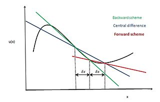
In applied mathematics, the central differencing scheme is a finite difference method that optimizes the approximation for the differential operator in the central node of the considered patch and provides numerical solutions to differential equations. It is one of the schemes used to solve the integrated convection–diffusion equation and to calculate the transported property Φ at the e and w faces, where e and w are short for east and west. The method's advantages are that it is easy to understand and implement, at least for simple material relations; and that its convergence rate is faster than some other finite differencing methods, such as forward and backward differencing. The right side of the convection-diffusion equation, which basically highlights the diffusion terms, can be represented using central difference approximation. To simplify the solution and analysis, linear interpolation can be used logically to compute the cell face values for the left side of this equation, which is nothing but the convective terms. Therefore, cell face values of property for a uniform grid can be written as:
Unsteady flows are characterized as flows in which the properties of the fluid are time dependent. It gets reflected in the governing equations as the time derivative of the properties are absent. For Studying Finite-volume method for unsteady flow there is some governing equations >
The upwind differencing scheme is a method used in numerical methods in computational fluid dynamics for convection–diffusion problems. This scheme is specific for Peclet number greater than 2 or less than −2
The convection–diffusion equation describes the flow of heat, particles, or other physical quantities in situations where there is both diffusion and convection or advection. For information about the equation, its derivation, and its conceptual importance and consequences, see the main article convection–diffusion equation. This article describes how to use a computer to calculate an approximate numerical solution of the discretized equation, in a time-dependent situation.
Finite volume method (FVM) is a numerical method. FVM in computational fluid dynamics is used to solve the partial differential equation which arises from the physical conservation law by using discretisation. Convection is always followed by diffusion and hence where convection is considered we have to consider combine effect of convection and diffusion. But in places where fluid flow plays a non-considerable role we can neglect the convective effect of the flow. In this case we have to consider more simplistic case of only diffusion. The general equation for steady convection-diffusion can be easily derived from the general transport equation for property by deleting transient.
In physical oceanography and fluid mechanics, the Miles-Phillips mechanism describes the generation of wind waves from a flat sea surface by two distinct mechanisms. Wind blowing over the surface generates tiny wavelets. These wavelets develop over time and become ocean surface waves by absorbing the energy transferred from the wind. The Miles-Phillips mechanism is a physical interpretation of these wind-generated surface waves. Both mechanisms are applied to gravity-capillary waves and have in common that waves are generated by a resonance phenomenon. The Miles mechanism is based on the hypothesis that waves arise as an instability of the sea-atmosphere system. The Phillips mechanism assumes that turbulent eddies in the atmospheric boundary layer induce pressure fluctuations at the sea surface. The Phillips mechanism is generally assumed to be important in the first stages of wave growth, whereas the Miles mechanism is important in later stages where the wave growth becomes exponential in time.
References
↑ Versteeg, H.K.; Malalasekera, W. (2007). An introduction to computational fluid dynamics: the finite volume method (2nded.). Harlow: Prentice Hall. ISBN9780131274983.
↑ Patankar, Suhas V. (1980). Numerical heat transfer and fluid flow (14. printing.ed.). Bristol, PA: Taylor & Francis. ISBN9780891165224.
This page is based on this Wikipedia article Text is available under the CC BY-SA 4.0 license; additional terms may apply. Images, videos and audio are available under their respective licenses.