In statistics, an estimator is a rule for calculating an estimate of a given quantity based on observed data: thus the rule, the quantity of interest and its result are distinguished. For example, the sample mean is a commonly used estimator of the population mean.
A parameter, generally, is any characteristic that can help in defining or classifying a particular system. That is, a parameter is an element of a system that is useful, or critical, when identifying the system, or when evaluating its performance, status, condition, etc.
In statistics, maximum likelihood estimation (MLE) is a method of estimating the parameters of an assumed probability distribution, given some observed data. This is achieved by maximizing a likelihood function so that, under the assumed statistical model, the observed data is most probable. The point in the parameter space that maximizes the likelihood function is called the maximum likelihood estimate. The logic of maximum likelihood is both intuitive and flexible, and as such the method has become a dominant means of statistical inference.

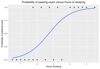
In statistics, the logistic model is a statistical model that models the log-odds of an event as a linear combination of one or more independent variables. In regression analysis, logistic regression estimates the parameters of a logistic model. In binary logistic regression there is a single binary dependent variable, coded by an indicator variable, where the two values are labeled "0" and "1", while the independent variables can each be a binary variable or a continuous variable. The corresponding probability of the value labeled "1" can vary between 0 and 1, hence the labeling; the function that converts log-odds to probability is the logistic function, hence the name. The unit of measurement for the log-odds scale is called a logit, from logistic unit, hence the alternative names. See § Background and § Definition for formal mathematics, and § Example for a worked example.
In mathematics, a Gaussian function, often simply referred to as a Gaussian, is a function of the base form and with parametric extension for arbitrary real constants a, b and non-zero c. It is named after the mathematician Carl Friedrich Gauss. The graph of a Gaussian is a characteristic symmetric "bell curve" shape. The parameter a is the height of the curve's peak, b is the position of the center of the peak, and c controls the width of the "bell".
In signal processing, a finite impulse response (FIR) filter is a filter whose impulse response is of finite duration, because it settles to zero in finite time. This is in contrast to infinite impulse response (IIR) filters, which may have internal feedback and may continue to respond indefinitely.
Cost estimation models are mathematical algorithms or parametric equations used to estimate the costs of a product or project. The results of the models are typically necessary to obtain approval to proceed, and are factored into business plans, budgets, and other financial planning and tracking mechanisms.

A sensor array is a group of sensors, usually deployed in a certain geometry pattern, used for collecting and processing electromagnetic or acoustic signals. The advantage of using a sensor array over using a single sensor lies in the fact that an array adds new dimensions to the observation, helping to estimate more parameters and improve the estimation performance. For example an array of radio antenna elements used for beamforming can increase antenna gain in the direction of the signal while decreasing the gain in other directions, i.e., increasing signal-to-noise ratio (SNR) by amplifying the signal coherently. Another example of sensor array application is to estimate the direction of arrival of impinging electromagnetic waves. The related processing method is called array signal processing. A third examples includes chemical sensor arrays, which utilize multiple chemical sensors for fingerprint detection in complex mixtures or sensing environments. Application examples of array signal processing include radar/sonar, wireless communications, seismology, machine condition monitoring, astronomical observations fault diagnosis, etc.
In statistics, econometrics, and signal processing, an autoregressive (AR) model is a representation of a type of random process; as such, it can be used to describe certain time-varying processes in nature, economics, behavior, etc. The autoregressive model specifies that the output variable depends linearly on its own previous values and on a stochastic term ; thus the model is in the form of a stochastic difference equation which should not be confused with a differential equation. Together with the moving-average (MA) model, it is a special case and key component of the more general autoregressive–moving-average (ARMA) and autoregressive integrated moving average (ARIMA) models of time series, which have a more complicated stochastic structure; it is also a special case of the vector autoregressive model (VAR), which consists of a system of more than one interlocking stochastic difference equation in more than one evolving random variable.
In statistics, the method of moments is a method of estimation of population parameters. The same principle is used to derive higher moments like skewness and kurtosis.
Cost estimation in software engineering is typically concerned with the financial spend on the effort to develop and test the software, this can also include requirements review, maintenance, training, managing and buying extra equipment, servers and software. Many methods have been developed for estimating software costs for a given project.
SEER for Software (SEER-SEM) is a project management application used to estimate resources required for software development.
Bootstrapping is a procedure for estimating the distribution of an estimator by resampling one's data or a model estimated from the data. Bootstrapping assigns measures of accuracy to sample estimates. This technique allows estimation of the sampling distribution of almost any statistic using random sampling methods.
Stochastic frontier analysis (SFA) is a method of economic modeling. It has its starting point in the stochastic production frontier models simultaneously introduced by Aigner, Lovell and Schmidt (1977) and Meeusen and Van den Broeck (1977).
In statistical signal processing, the goal of spectral density estimation (SDE) or simply spectral estimation is to estimate the spectral density of a signal from a sequence of time samples of the signal. Intuitively speaking, the spectral density characterizes the frequency content of the signal. One purpose of estimating the spectral density is to detect any periodicities in the data, by observing peaks at the frequencies corresponding to these periodicities.
Katz back-off is a generative n-gram language model that estimates the conditional probability of a word given its history in the n-gram. It accomplishes this estimation by backing off through progressively shorter history models under certain conditions. By doing so, the model with the most reliable information about a given history is used to provide the better results.
The Larson–Miller relation, also widely known as the Larson–Miller parameter and often abbreviated LMP, is a parametric relation used to extrapolate experimental data on creep and rupture life of engineering materials.
In software development, effort estimation is the process of predicting the most realistic amount of effort required to develop or maintain software based on incomplete, uncertain and noisy input. Effort estimates may be used as input to project plans, iteration plans, budgets, investment analyses, pricing processes and bidding rounds.

In statistics, errors-in-variables models or measurement error models are regression models that account for measurement errors in the independent variables. In contrast, standard regression models assume that those regressors have been measured exactly, or observed without error; as such, those models account only for errors in the dependent variables, or responses.
In statistics, the variance function is a smooth function that depicts the variance of a random quantity as a function of its mean. The variance function is a measure of heteroscedasticity and plays a large role in many settings of statistical modelling. It is a main ingredient in the generalized linear model framework and a tool used in non-parametric regression, semiparametric regression and functional data analysis. In parametric modeling, variance functions take on a parametric form and explicitly describe the relationship between the variance and the mean of a random quantity. In a non-parametric setting, the variance function is assumed to be a smooth function.


