In physics, a conservation law states that a particular measurable property of an isolated physical system does not change as the system evolves over time. Exact conservation laws include conservation of mass-energy, conservation of linear momentum, conservation of angular momentum, and conservation of electric charge. There are also many approximate conservation laws, which apply to such quantities as mass, parity, lepton number, baryon number, strangeness, hypercharge, etc. These quantities are conserved in certain classes of physics processes, but not in all.

In the field of complex analysis in mathematics, the Cauchy–Riemann equations, named after Augustin Cauchy and Bernhard Riemann, consist of a system of two partial differential equations which form a necessary and sufficient condition for a complex function of a complex variable to be complex differentiable.
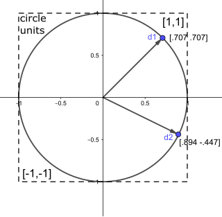
In mathematics, a unit vector in a normed vector space is a vector of length 1. A unit vector is often denoted by a lowercase letter with a circumflex, or "hat", as in .
The finite volume method (FVM) is a method for representing and evaluating partial differential equations in the form of algebraic equations. In the finite volume method, volume integrals in a partial differential equation that contain a divergence term are converted to surface integrals, using the divergence theorem. These terms are then evaluated as fluxes at the surfaces of each finite volume. Because the flux entering a given volume is identical to that leaving the adjacent volume, these methods are conservative. Another advantage of the finite volume method is that it is easily formulated to allow for unstructured meshes. The method is used in many computational fluid dynamics packages. "Finite volume" refers to the small volume surrounding each node point on a mesh.

In fluid dynamics, the Euler equations are a set of quasilinear partial differential equations governing adiabatic and inviscid flow. They are named after Leonhard Euler. In particular, they correspond to the Navier–Stokes equations with zero viscosity and zero thermal conductivity.
In mathematics and computing, the Levenberg–Marquardt algorithm, also known as the damped least-squares (DLS) method, is used to solve non-linear least squares problems. These minimization problems arise especially in least squares curve fitting. The LMA interpolates between the Gauss–Newton algorithm (GNA) and the method of gradient descent. The LMA is more robust than the GNA, which means that in many cases it finds a solution even if it starts very far off the final minimum. For well-behaved functions and reasonable starting parameters, the LMA tends to be slower than the GNA. LMA can also be viewed as Gauss–Newton using a trust region approach.

In applied statistics, total least squares is a type of errors-in-variables regression, a least squares data modeling technique in which observational errors on both dependent and independent variables are taken into account. It is a generalization of Deming regression and also of orthogonal regression, and can be applied to both linear and non-linear models.

The Gauss–Newton algorithm is used to solve non-linear least squares problems, which is equivalent to minimizing a sum of squared function values. It is an extension of Newton's method for finding a minimum of a non-linear function. Since a sum of squares must be nonnegative, the algorithm can be viewed as using Newton's method to iteratively approximate zeroes of the components of the sum, and thus minimizing the sum. In this sense, the algorithm is also an effective method for solving overdetermined systems of equations. It has the advantage that second derivatives, which can be challenging to compute, are not required.
In mathematics, a hyperbolic partial differential equation of order is a partial differential equation (PDE) that, roughly speaking, has a well-posed initial value problem for the first derivatives. More precisely, the Cauchy problem can be locally solved for arbitrary initial data along any non-characteristic hypersurface. Many of the equations of mechanics are hyperbolic, and so the study of hyperbolic equations is of substantial contemporary interest. The model hyperbolic equation is the wave equation. In one spatial dimension, this is
In numerical analysis and computational fluid dynamics, Godunov's scheme is a conservative numerical scheme, suggested by Sergei Godunov in 1959, for solving partial differential equations. One can think of this method as a conservative finite volume method which solves exact, or approximate Riemann problems at each inter-cell boundary. In its basic form, Godunov's method is first order accurate in both space and time, yet can be used as a base scheme for developing higher-order methods.
In the study of partial differential equations, the MUSCL scheme is a finite volume method that can provide highly accurate numerical solutions for a given system, even in cases where the solutions exhibit shocks, discontinuities, or large gradients. MUSCL stands for Monotonic Upstream-centered Scheme for Conservation Laws, and the term was introduced in a seminal paper by Bram van Leer. In this paper he constructed the first high-order, total variation diminishing (TVD) scheme where he obtained second order spatial accuracy.
In statistics, the multivariate t-distribution is a multivariate probability distribution. It is a generalization to random vectors of the Student's t-distribution, which is a distribution applicable to univariate random variables. While the case of a random matrix could be treated within this structure, the matrix t-distribution is distinct and makes particular use of the matrix structure.

A Riemann solver is a numerical method used to solve a Riemann problem. They are heavily used in computational fluid dynamics and computational magnetohydrodynamics.
In applied mathematics, discontinuous Galerkin methods (DG methods) form a class of numerical methods for solving differential equations. They combine features of the finite element and the finite volume framework and have been successfully applied to hyperbolic, elliptic, parabolic and mixed form problems arising from a wide range of applications. DG methods have in particular received considerable interest for problems with a dominant first-order part, e.g. in electrodynamics, fluid mechanics and plasma physics.
In computational fluid dynamics, shock-capturing methods are a class of techniques for computing inviscid flows with shock waves. The computation of flow containing shock waves is an extremely difficult task because such flows result in sharp, discontinuous changes in flow variables such as pressure, temperature, density, and velocity across the shock.
Non-linear least squares is the form of least squares analysis used to fit a set of m observations with a model that is non-linear in n unknown parameters (m ≥ n). It is used in some forms of nonlinear regression. The basis of the method is to approximate the model by a linear one and to refine the parameters by successive iterations. There are many similarities to linear least squares, but also some significant differences. In economic theory, the non-linear least squares method is applied in (i) the probit regression, (ii) threshold regression, (iii) smooth regression, (iv) logistic link regression, (v) Box–Cox transformed regressors ().
In estimation theory, the extended Kalman filter (EKF) is the nonlinear version of the Kalman filter which linearizes about an estimate of the current mean and covariance. In the case of well defined transition models, the EKF has been considered the de facto standard in the theory of nonlinear state estimation, navigation systems and GPS.
In fluid dynamics, Airy wave theory gives a linearised description of the propagation of gravity waves on the surface of a homogeneous fluid layer. The theory assumes that the fluid layer has a uniform mean depth, and that the fluid flow is inviscid, incompressible and irrotational. This theory was first published, in correct form, by George Biddell Airy in the 19th century.
The Lax–Friedrichs method, named after Peter Lax and Kurt O. Friedrichs, is a numerical method for the solution of hyperbolic partial differential equations based on finite differences. The method can be described as the FTCS scheme with a numerical dissipation term of 1/2. One can view the Lax–Friedrichs method as an alternative to Godunov's scheme, where one avoids solving a Riemann problem at each cell interface, at the expense of adding artificial viscosity.
In mathematics, the method of steepest descent or saddle-point method is an extension of Laplace's method for approximating an integral, where one deforms a contour integral in the complex plane to pass near a stationary point, in roughly the direction of steepest descent or stationary phase. The saddle-point approximation is used with integrals in the complex plane, whereas Laplace’s method is used with real integrals.


