SP-DEVS

Last updated

SP-DEVS abbreviating "Schedule-Preserving Discrete Event System Specification" is a formalism for modeling and analyzing discrete event systems in both simulation and verification ways. SP-DEVS also provides modular and hierarchical modeling features which have been inherited from the Classic DEVS.

Contents

History

SP-DEVS has been designed to support verification analysis of its networks by guaranteeing to obtain a finite-vertex reachability graph of the original networks, which had been an open problem of DEVS formalism for roughly 30 years. To get such a reachability graph of its networks, SP-DEVS has been imposed the three restrictions:

  1. finiteness of event sets and state set,
  2. the lifespan of a state can be scheduled by a rational number or infinity, and
  3. preserving the internal schedule from any external events.

Thus, SP-DEVS is a sub-class of both DEVS and FD-DEVS. These three restrictions lead that SP-DEVS class is closed under coupling even though the number of states are finite. This property enables a finite-vertex graph-based verification for some qualitative properties and quantitative property, even with SP-DEVS coupled models.

Crosswalk Controller Example

System Requirements
Fig. 1. Crosswalk System Crosswalk.svg
Fig. 1. Crosswalk System
Fig. 2. SP-DEVS model for Crosswalk Light Controller SP-DEVS controller for crosswalk lights.svg
Fig. 2. SP-DEVS model for Crosswalk Light Controller

Consider a crosswalk system. Since a red light (resp. don't-walk light) behaves the opposite way of a green light (resp. walk light), for simplicity, we consider just two lights: a green light (G) and a walk light (W); and one push button as shown in Fig. 1. We want to control two lights of G and W with a set of timing constraints.

To initialize two lights, it takes 0.5 seconds to turn G on and 0.5 seconds later, W gets off. Then, every 30 seconds, there is a chance that G becomes off and W on if someone pushed the push button. For a safety reason, W becomes on two seconds after G got off. 26 seconds later, W gets off and then two seconds later G gets back on. These behaviors repeats.

Controller Design

To build a controller for above requirements, we can consider one input event 'push-button' (abbreviated by ?p) and four output events 'green-on' (!g:1), 'green-off' (!g:0), 'walk-on' (!w:1) and 'walk-off (!w:0) which will be used as commands signals for the green light and the walk light. As a set of states of the controller, we considers 'booting-green' (BG), 'booting-walk' (BW), 'green-on' (G), 'green-to-red' (GR), 'red-on' (R), 'walk-on' (W), 'delay' (D). Let's design the state transitions as shown in Fig. 2. Initially, the controller starts at BG whose lifespan is 0.5 seconds. After the lifespan, it moves to BW state at this moment, it generates the 'green-on' event, too. After 0.5 seconds staying at BW, it moves to G state whose lifespan is 30 seconds. The controller can keep staying at G by looping G to G without generating any output event or can move to GR state when it receives the external input event ?p. But, the actual staying time at GR is the remaining time for looping at G. From GR, it moves to R state with generating an output event !g:0 and its R state last two seconds then it will move to W state with output event !w:1. 26 seconds later, it moves to D state with generating !w:0 and after staying 2 seconds at D, it moves back to G with output event !g:1.

Atomic SP-DEVS

Formal Definition

The above controller for crosswalk lights can be modeled by an atomic SP-DEVS model. Formally, an atomic SP-DEVS is a 7-tuple

where

  • is a finite set of input events;
  • is a finite set of output events;
  • is a finite set of states;
  • is the initial state;
  • is the time advanced function which defines the lifespan of a state where is the set of non-negative rational numbers plus infinity.
  • is the external transition function which defines how an input event changes a state of the system.
  • is the output and internal transition function where and denotes the silent event. The output and internal transition function defines how a state generates an output event, at the same time, how the state changes internally. [1]
Formal Representation of Crosswalk Controller

The above controller shown in Fig. 2 can be written as where ={?p}; ={!g:0, !g:1, !w:0, !w:1}; ={BG, BW, G, GR, R, W, D}; =BG, (BG)=0.5,(BW)=0.5, (G)=30, (GR)=30,(R)=2, (W)=26, (D)=2; (G,?p)=GR, (s,?p)=s if s G; (BG)=(!g:1, BW), (BW)=(!w:0, G),(G)=(, G), (GR)=(!g:0, R), (R)=(!w:1, W), (W)=(!w:0, D), (D)=(!g:1, G);

Behaviors of a SP-DEVS model

Fig. 3. Event Segment and its State Trajectory of SP-DEVS model SPDEVS-Trajectory.JPG
Fig. 3. Event Segment and its State Trajectory of SP-DEVS model

To captured the dynamics of an atomic SP-DEVS, we need to introduce two variables associated to time. One is the lifespan, the other is the elapsed time since the last resetting. Let be the lifespan which is not continuously increasing but set by when a discrete event happens. Let denote the elapsed time which is continuously increasing over time if there is no resetting.

Fig.3. shows a state trajectory associated with an event segment of the SP-DEVS model shown in Fig. 2. The top of Fig.3. shows an event trajectory in which the horizontal axis is a time axis so it shows an event occurs at a certain time, for example, !g:1 occurs at 0.5 and !w:0 at 1.0 time unit, and so on. The bottom of Fig. 3 shows the state trajectory associated with the above event segment in which the state is associated with its lifespan and its elapsed time in the form of . For example, (G, 30, 11) denotes that the state is G, its lifespan is and the elapsed time is 11 time units. The line segments of the bottom of Fig. 3 shows the time flow of the elapsed time which is the only one continuous variable in SP-DEVS.

One interesting feature of SF-DEVS might be the preservation of schedule the restriction (3) of SP-DEVS which is drawn at time 47 in Fig. 3. when the external event ?p happens. At this moment, even though the state can change from G to GR, the elapsed time does not change so the line segment is not broken at time 47 and can grow up to which is 30 in this example. Due to this preservation of the schedule from input events as well as the restriction of the time advance to the non-negative rational number (see restriction (2) above), the height of every saw can be a non-negative rational number or infinity (as shown in the bottom of Fig. 3.) in a SP-DEVS model.

SP-DEVS is a sub-class of DEVS

A SP-DEVS model, is DEVS where

Advantages

The property of non-negative rational-valued lifespans which are not changed by input events along with finite numbers of states and events guarantees that the behavior of SP-DEVS networks can be abstracted as an equivalent finite-vertex reachability graph by abstracting the infinitely-many values of the elapsed times.

To abstract the infinitely-many cases of elapsed times for each components of SP-DEVS networks, a time-abstraction method, called the time-line abstraction has been introduced [Hwang05],[HCZF07] in which the orders and relative difference of schedules are preserved. By using the time-line abstraction technique, the behavior of any SP-DEVS network can be abstracted as a reachability graph whose numbers of vertices and edges are finite.

As a qualitative property, safety of a SP-DEVS network is decidable by (1) generating the finite-vertex reachability graph of the given network and (2) checking whether some bad states are reachable or not [Hwang05].

As a qualitative property, liveness of a SP-DEVS network is decidable by (1) generating the finite-vertex reachability graph (RG) of the given network, (2) from RG, generating kernel directed acyclic graph (KDAG) in which a vertex is strongly connected component, and (3) checking if a vertex of KDAG contains a state transition cycle which contains a set of liveness states[Hwang05].

As a quantitative property, minimum and maximum processing time bounds from two events in SP-DEVS networks can be computed by (1) generating the finite-vertex reachability graph and (2.a) by finding the shortest paths for the minimum processing time bound and (2.b) by finding the longest paths (if available) for the maximum processing time bound [HCZF07].

Disadvantages

Let a total state of a SP-DEVS model be passive if ; otherwise, it be active.

One of known SP-DEVS's limitation is a phenomenon that "once an SP-DEVS model becomes passive, it never returns to become active (OPNA)". This phenomenon was found first at [Hwang 05b] although it was originally called ODNR ("once it dies, it never returns."). The reason why this one happens is because of the restriction (3) above in which no input event can change the schedule so the passive state can not be awaken into the active state.

For example, the toaster models drawn in Fig. 3(b) are not SP-DEVS because the total state associated with "idle" (I), is passive but it moves to an active state, "toast" (T) whose toating time is 20 seconds or 40 seconds. Actually, the model shown in Fig. 3(b) is FD-DEVS.

Tool

There is an open source library, called DEVS# at http://xsy-csharp.sourceforge.net/DEVSsharp/, that supports some algorithms for finding safeness and liveness as well as Min/Max processing time bounds.

Footnotes

  1. can be divided into two functions: and as in [ZKP00].

Related Research Articles

Convolution Binary mathematical operation on functions

In mathematics, convolution is a mathematical operation on two functions that produces a third function that expresses how the shape of one is modified by the other. The term convolution refers to both the result function and to the process of computing it. It is defined as the integral of the product of the two functions after one is reversed and shifted. The integral is evaluated for all values of shift, producing the convolution function.

Feynman diagram Pictorial representation of the behavior of subatomic particles

In theoretical physics, a Feynman diagram is a pictorial representation of the mathematical expressions describing the behavior and interaction of subatomic particles. The scheme is named after American physicist Richard Feynman, who introduced the diagrams in 1948. The interaction of subatomic particles can be complex and difficult to understand; Feynman diagrams give a simple visualization of what would otherwise be an arcane and abstract formula. According to David Kaiser, "Since the middle of the 20th century, theoretical physicists have increasingly turned to this tool to help them undertake critical calculations. Feynman diagrams have revolutionized nearly every aspect of theoretical physics." While the diagrams are applied primarily to quantum field theory, they can also be used in other fields, such as solid-state theory. Frank Wilczek wrote that the calculations which won him the 2004 Nobel Prize in Physics "would have been literally unthinkable without Feynman diagrams, as would [Wilczek's] calculations that established a route to production and observation of the Higgs particle."
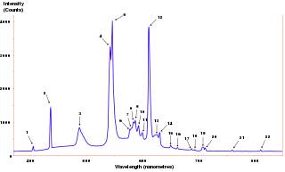
Spectral density Relative importance of certain frequencies in a composite signal

The power spectrum of a time series describes the distribution of power into frequency components composing that signal. According to Fourier analysis, any physical signal can be decomposed into a number of discrete frequencies, or a spectrum of frequencies over a continuous range. The statistical average of a certain signal or sort of signal as analyzed in terms of its frequency content, is called its spectrum.

Discretization Process of transferring continuous functions into discrete counterparts

In applied mathematics, discretization is the process of transferring continuous functions, models, variables, and equations into discrete counterparts. This process is usually carried out as a first step toward making them suitable for numerical evaluation and implementation on digital computers. Dichotomization is the special case of discretization in which the number of discrete classes is 2, which can approximate a continuous variable as a binary variable.

Short-time Fourier transform Fourier-related transform suited to signals that change rather quickly in time

The Short-time Fourier transform (STFT), is a Fourier-related transform used to determine the sinusoidal frequency and phase content of local sections of a signal as it changes over time. In practice, the procedure for computing STFTs is to divide a longer time signal into shorter segments of equal length and then compute the Fourier transform separately on each shorter segment. This reveals the Fourier spectrum on each shorter segment. One then usually plots the changing spectra as a function of time, known as a spectrogram or waterfall plot, such as commonly used in Software Defined Radio (SDR) based spectrum displays. Full bandwidth displays covering the whole range of an SDR commonly use Fast Fourier Transforms (FFTs) with 2^24 points on desktop computers.

Proper time Elapsed time between two events as measured by a clock that passes through both events

In relativity, proper time along a timelike world line is defined as the time as measured by a clock following that line. It is thus independent of coordinates, and is a Lorentz scalar. The proper time interval between two events on a world line is the change in proper time. This interval is the quantity of interest, since proper time itself is fixed only up to an arbitrary additive constant, namely the setting of the clock at some event along the world line.

Abstract simplicial complex

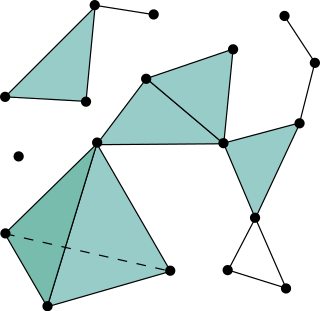
In combinatorics, an abstract simplicial complex (ASC), often called an abstract complex or just a complex, is a family of sets that is closed under taking subsets, i.e., every subset of a set in the family is also in the family. It is a purely combinatorial description of the geometric notion of a simplicial complex. For example, in a 2-dimensional simplicial complex, the sets in the family are the triangles, their edges, and their vertices.

Linear time-invariant system Mathematical model

In system analysis, among other fields of study, a linear time-invariant system is a system that produces an output signal from any input signal subject to the constraints of linearity and time-invariance; these terms are briefly defined below. These properties apply to many important physical systems, in which case the response y(t) of the system to an arbitrary input x(t) can be found directly using convolution: y(t) = x(t) ∗ h(t) where h(t) is called the system's impulse response and ∗ represents convolution. What's more, there are systematic methods for solving any such system, whereas systems not meeting both properties are generally more difficult to solve analytically. A good example of an LTI system is any electrical circuit consisting of resistors, capacitors, inductors and linear amplifiers.

The random walk hypothesis is a financial theory stating that stock market prices evolve according to a random walk and thus cannot be predicted.

Wigner distribution function

The Wigner distribution function (WDF) is used in signal processing as a transform in time-frequency analysis.

DEVS abbreviating Discrete Event System Specification is a modular and hierarchical formalism for modeling and analyzing general systems that can be discrete event systems which might be described by state transition tables, and continuous state systems which might be described by differential equations, and hybrid continuous state and discrete event systems. DEVS is a timed event system.

FD-DEVS is a formalism for modeling and analyzing discrete event dynamic systems in both simulation and verification ways. FD-DEVS also provides modular and hierarchical modeling features which have been inherited from Classic DEVS.

Triadic closure

Triadic closure is a concept in social network theory, first suggested by German sociologist Georg Simmel in his 1908 book Soziologie [Sociology: Investigations on the Forms of Sociation]. Triadic closure is the property among three nodes A, B, and C, that if the connections A-B and A-C exist, there is a tendency for the new connection B-C to be formed. Triadic closure can be used to understand and predict the growth of networks, although it is only one of many mechanisms by which new connections are formed in complex networks.

Black–Scholes equation

In mathematical finance, the Black–Scholes equation is a partial differential equation (PDE) governing the price evolution of a European call or European put under the Black–Scholes model. Broadly speaking, the term may refer to a similar PDE that can be derived for a variety of options, or more generally, derivatives.

The behavior of a given DEVS model is a set of sequences of timed events including null events, called event segments, which make the model move from one state to another within a set of legal states. To define it this way, the concept of a set of illegal state as well a set of legal states needs to be introduced.

Abelian sandpile model Cellular automaton

The Abelian sandpile model (ASM) is the more popular name of the original Bak–Tang–Wiesenfeld model (BTW). BTW model was the first discovered example of a dynamical system displaying self-organized criticality. It was introduced by Per Bak, Chao Tang and Kurt Wiesenfeld in a 1987 paper.

Given an atomic DEVS model, simulation algorithms are methods to generate the model's legal behaviors which are trajectories not to reach to illegal states.. [Zeigler84] originally introduced the algorithms that handle time variables related to lifespan and elapsed time by introducing two other time variables, last event time, , and next event time with the following relations:

Laser linewidth is the spectral linewidth of a laser beam.

In mathematics, the infinity Laplace operator is a 2nd-order partial differential operator, commonly abbreviated . It is alternately defined by

In mathematics, the Fuglede−Kadison determinant of an invertible operator in a finite factor is a positive real number associated with it. It defines a multiplicative homomorphism from the set of invertible operators to the set of positive real numbers. The Fuglede−Kadison determinant of an operator is often denoted by .

References