Spectral estimation of multidimensional signals

Last updated June 01, 2020

Power spectral estimation forms the basis for distinguishing and tracking signals in the presence of noise and extracting information from available data. One dimensional signals are expressed in terms of a single domain while multidimensional signals are represented in wave vector and frequency spectrum. Therefore, spectral estimation in the case of multidimensional signals gets a bit tricky.

Motivation

Multidimensional spectral estimation has gained popularity because of its application in fields like medicine, aerospace, sonar, radar, bio informatics and geophysics. In the recent past, a number of methods have been suggested to design models with finite parameters to estimate the power spectrum of multidimensional signals. In this article, we will be looking into the basics of methods used to estimate the power spectrum of multidimensional signals.

Applications

There are many applications of spectral estimation of multi-D signals such as classification of signals as low pass, high pass, pass band and stop band. It is also used in compression and coding of audio and video signals, beam forming and direction finding in radars,^[1] Seismic data estimation and processing, array of sensors and antennas and vibrational analysis. In the field of radio astronomy,^[1] it is used to synchronize the outputs of an array of telescopes.

Basic Concepts

In a single dimensional case, a signal is characterized by an amplitude and a time scale. The basic concepts involved in spectral estimation include autocorrelation, multi-D Fourier transform, mean square error and entropy.^[2] When it comes to multidimensional signals, there are two main approaches: use a bank of filters or estimate the parameters of the random process in order to estimate the power spectrum.

spectral estimation techniques Spectral estimation techniques.jpg — spectral estimation techniques

Methods

Classical Estimation Theory

It is a technique to estimate the power spectrum of a single dimensional or a multidimensional signal as it cannot be calculated accurately. Given are samples of a wide sense stationary random process and its second order statistics (measurements).The estimates are obtained by applying a multidimensional Fourier transform of the autocorrelation function of the random signal. The estimation begins by calculating a periodogram which is obtained by squaring the magnitude of the multidimensional Fourier transform of the measurements ri(n). The spectral estimates obtained from the periodogram have a large variance in amplitude for consecutive periodogram samples or in wavenumber. This problem is resolved using techniques that constitute the classical estimation theory. They are as follows: 1.Bartlett suggested a method that averages the spectral estimates to calculate the power spectrum. The measurements are divided into equally spaced segments in time and an average is taken. This gives a better estimate.^[3] 2.Based on the wavenumber and index of the receiver/output we can partition the segments. This increases the spectral estimates and decreases the variances between consecutive segments. 3.Welch suggested that we should divide the measurements using data window functions, calculate a periodogram, average them to get a spectral estimate and calculate the power spectrum using Fast Fourier Transform (FFT). This increases the computational speed.^[4] 4.Smoothing window will help us smoothen the estimate by multiplying the periodogram with a smoothening spectrum. Wider the main lobe of the smoothening spectrum, smoother it becomes at the cost of frequency resolution.^[2] $P\left(K_{x},w\right)=\int _{-\infty }^{\infty }\int _{-\infty }^{\infty }\varphi _{ss}\left(x,t\right)\ e^{-j\left(wt-k'x\right)}\,dx\,dt$

$\varphi _{ss}\left(x,t\right)=s\left[\left(\xi ,\tau \right)s^{*}\left(\xi -x,\tau -t\right)\right]$ ^[2]

$P_{B}\left(w\right)={\frac {1}{detN}}\sum _{l}|\sum _{n}\ x\left(n+MI\right)\ e^{-j\left(w'n\right)}|^{2}$ Bartlett's case ^[2]

$P_{M}\left(w\right)={\frac {1}{detN}}|\sum _{n}\ g\left(n\right)\ x\left(n\right)\ e^{-j\left(w'n\right)}|^{2}$ Modified periodogram ^[2]

$P_{W}\left(w\right)={\frac {1}{detN}}\sum _{l}|\sum _{n}\ g\left(n\right)\ x\left(n+MI\right)\ e^{-j\left(w'n\right)}|^{2}$ Welch's case ^[2]

Advantages: Straightforward method involving Fourier transforms.

Limitations: 1.Since some of the above methods sample the sequence in time, the frequency resolution is reduced (aliasing). 2.Number of instances of a wide sense stationary random process are less which makes it difficult to calculate the estimates accurately.

High Resolution Spectral Estimations

This method gives a better estimate whose frequency resolution is higher than the classical estimation theory. In the high resolution estimation method we use a variable wavenumber window which allows only certain wavenumbers and suppresses the others. Capon’s ^[5] work helped us establish an estimation method by using wavenumber-frequency components. This results in an estimate with a higher frequency resolution. It is similar to maximum likelihood method as the optimization tool used is similar.

Assumption: The output obtained from the sensors is a wide sense stationary random process with zero mean.^[6]

$P_{C}\left(K_{o}x,w_{o}\right)=E\left[|y\left(i,n\right)|^{2}\right]={\frac {1}{\sum _{\alpha =0}^{N-1}\sum _{\beta =0}^{M-1}\sum _{l=0}^{N-1}\sum _{m=0}^{M-1}\psi _{e}\left(l,\alpha ;m,\beta \right)}}$ ^[2]

Advantages: 1.Higher frequency resolution compare to other existing methods. 2.Better frequency estimate since we are using a variable wavenumber window as compared to classical method which uses a fixed wavenumber window. 3.Faster Computational speed as it uses FFT.

Separable Spectral Estimator

^[1]

In this type of estimation, we select the multidimensional signal to be a separable function. Because of this property we will be able to view the Fourier analysis taking place in multiple dimensions successively. A time delay in the magnitude squaring operation will help us process the Fourier transformation in each dimension. A Discrete time Multidimensional Fourier transform is applied along each dimension and in the end a maximum entropy estimator is applied and the magnitude is squared.

Advantages: 1. The Fourier analysis is flexible as the signal is separable. 2.It preserves the phase components of every dimension unlike other spectral estimators.

All-pole Spectral Modelling

^[2]
This method is an extension of a 1-D technique called Autoregressive spectral estimation. In autoregressive models, the output variables depend linearly on its own previous values. In this model, the estimation of power spectrum is reduced to estimating the coefficients from the autocorrelation coefficients of the random process which are assumed to be known for a specific region. The power spectrum $P_{A}(k_{x},w)$ of a random process $r(i,n)$ is given by:-

$P_{A}\left(k_{x},w\right)=P_{e}\left(k_{x},w\right)|{\frac {1}{1-A\left(k_{x},w\right)}}|^{2}$ ^[2]

Where $P_{e}\left(k_{x},w\right)$ is the power spectrum of a random process $e(i,n)$ , which is given as the input to a system with a transfer function $|{\frac {1}{1-A\left(k_{x},w\right)}}|$ to obtain $r(i,n)$ ^[2]

And $A\left(k_{x},w\right)=\sum _{p=o}^{N-1}\sum _{q=0}^{M-1}a(p,q)exp(jk_{x}p-jwq)$ ^[2]
Therefore, the power estimation reduces to estimation of coefficients of $a\left(p,q\right)$ from the auto correlation function $\varphi \left(l,m\right)$ of the random process. The coefficients can also be estimated using the linear prediction formulation which deals with minimization of mean square error between the actual random signal and predicted values of the random signal.

Limitations:-
1. In 1-D we have the same number of linear equations with the same number of unknowns because of the autocorrelation matching property. But it may not be possible in multi-D ^[2] since the set of parameters does not contain enough degrees of freedom to match autocorrelation coefficients.
2. We assume that the array of coefficients is limited to a certain area.
3. In 1-D formulation of linear prediction, the inverse filter has minimum phase property thus proving that the filter is stable. It is not always necessarily true in multi-D case.
4. In 1-D formulation, the autocorrelation matrix is positive definite but positive definite extension may not exist in the case of multi-D.

Maximum Entropy Spectral Estimation

In this method of spectral estimation, we try to find the spectral estimate whose inverse Fourier transform matches the known auto correlation coefficients. We maximize the entropy of the spectral estimate such that it matches the autocorrelation coefficients.^[2] The entropy equation is given as $H={\frac {1}{4\pi ^{2}}}\int _{-\pi }^{\pi }\int _{-\pi }^{\pi }logP\left(k_{x},w\right)dk_{x}dw$ ^[1]^[2]
The power spectrum $P\left(k,w\right)$ can be expressed as a sum of known autocorrelation coefficients and unknown autocorrelation coefficients. By adjusting the values of unconstrained coefficients, the entropy can be maximized.
The max entropy is of the form $P_{ME}={\frac {1}{\sum _{l}\sum _{m}\lambda \left(l,m\right)exp\left(jk_{x}l-jwm\right)}}$ ^[1]^[2]
λ(l,m) must be chosen such that known autocorrelation coefficients are matched.

Limitations:-
1.It has constrained optimization. It can be overcome by using the method of Lagrange multipliers.^[2]
2. All pole spectral estimate is not the solution to maximum entropy in multidimensional case as it is in the case of 1-D. This is because the all pole spectral model does not contain enough degree of freedom to match the know autocorrelation coefficients.

Advantages and Disadvantages:-
The advantage of this estimator is that errors in measuring or estimating the known autocorrelation coefficients can be taken into account since exact match is not required.
The disadvantage is that too many computations are required.

Improved Maximum Likelihood Method(IMLM)

This is a relatively new approach. Improved maximum likelihood method (IMLM) is a combination of two MLM(maximum likelihood) estimators.^[1]^[7] The improved maximum likelihood of two 2-dimensional arrays A and B at a wave number k( gives information about the orientation of the array in space) is given by the relation:-
$IMLM\left(k:A,B\right)={\frac {1}{{\frac {1}{MLM\left(k:A\right)}}-{\frac {1}{MLM\left(k:B\right)}}}}$ ^[7]^[8]

Array B is a subset of A. Therefore, assuming that A>B, if there is a difference between the MLM of A and MLM of B then significant part of the estimated spectral energy at the frequency may be due to power leakage from other frequencies. The de-emphasis of MLM of A may improve spectral estimate. This is accomplished by multiplying by a weighted function which is smaller when there is a greater difference between MLA of B and MLA of A.
. $IMLM\left(k:A,B\right)={\frac {MLM\left(k:A\right)MLM\left(k:B\right)}{MLM\left(k:B\right)-MLM\left(k:A\right)}}$
$IMLM\left(k:A,B\right)=MLM\left(k:A\right)W_{AB}\left(k\right)$
where $W_{AB}\left(k\right)$ is the weighting function and is given by the expression:- $W_{AB}\left(k\right)={\frac {MLM\left(k:B\right)}{MLM\left(k:B\right)-MLM\left(k:A\right)}}$ ^[7]

Advantages:-
1. Used as an alternative to MLM or MEM(Maximum Entropy Method/principle of maximum entropy)
2. IMLM has better resolution than MLM and it requires lesser number of computations when compared to MEM ^[7]^[8]

Related Research Articles

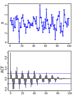
Autocorrelation, also known as serial correlation, is the correlation of a signal with a delayed copy of itself as a function of delay. Informally, it is the similarity between observations as a function of the time lag between them. The analysis of autocorrelation is a mathematical tool for finding repeating patterns, such as the presence of a periodic signal obscured by noise, or identifying the missing fundamental frequency in a signal implied by its harmonic frequencies. It is often used in signal processing for analyzing functions or series of values, such as time domain signals.

In mathematics, the discrete Fourier transform (DFT) converts a finite sequence of equally-spaced samples of a function into a same-length sequence of equally-spaced samples of the discrete-time Fourier transform (DTFT), which is a complex-valued function of frequency. The interval at which the DTFT is sampled is the reciprocal of the duration of the input sequence. An inverse DFT is a Fourier series, using the DTFT samples as coefficients of complex sinusoids at the corresponding DTFT frequencies. It has the same sample-values as the original input sequence. The DFT is therefore said to be a frequency domain representation of the original input sequence. If the original sequence spans all the non-zero values of a function, its DTFT is continuous, and the DFT provides discrete samples of one cycle. If the original sequence is one cycle of a periodic function, the DFT provides all the non-zero values of one DTFT cycle.

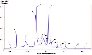
The power spectrum $of a time series describes the distribution of power into frequency components composing that signal. According to Fourier analysis, any physical signal can be decomposed into a number of discrete frequencies, or a spectrum of frequencies over a continuous range. The statistical average of a certain signal or sort of signal as analyzed in terms of its frequency content, is called its spectrum.$

Window function function used in signal processing

In signal processing and statistics, a window function is a mathematical function that is zero-valued outside of some chosen interval, normally symmetric around the middle of the interval, usually near a maximum in the middle, and usually tapering away from the middle. Mathematically, when another function or waveform/data-sequence is "multiplied" by a window function, the product is also zero-valued outside the interval: all that is left is the part where they overlap, the "view through the window". Equivalently, and in actual practice, the segment of data within the window is first isolated, and then only that data is multiplied by the window function values. Thus, tapering, not segmentation, is the main purpose of window functions.

In signal processing, a periodogram is an estimate of the spectral density of a signal. The term was coined by Arthur Schuster in 1898. Today, the periodogram is a component of more sophisticated methods. It is the most common tool for examining the amplitude vs frequency characteristics of FIR filters and window functions. FFT spectrum analyzers are also implemented as a time-sequence of periodograms.

Welch's method, named after Peter D. Welch, is an approach for spectral density estimation. It is used in physics, engineering, and applied mathematics for estimating the power of a signal at different frequencies. The method is based on the concept of using periodogram spectrum estimates, which are the result of converting a signal from the time domain to the frequency domain. Welch's method is an improvement on the standard periodogram spectrum estimating method and on Bartlett's method, in that it reduces noise in the estimated power spectra in exchange for reducing the frequency resolution. Due to the noise caused by imperfect and finite data, the noise reduction from Welch's method is often desired.

In mathematics, the discrete-time Fourier transform (DTFT) is a form of Fourier analysis that is applicable to a sequence of values.

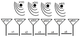
Array processing is a wide area of research in the field of signal processing that extends from the simplest form of 1 dimensional line arrays to 2 and 3 dimensional array geometries. Array structure can be defined as a set of sensors that are spatially separated, e.g. radio antenna and seismic arrays. The sensors used for a specific problem may vary widely, for example microphones, accelerometers and telescopes. However, many similarities exist, the most fundamental of which may be an assumption of wave propagation. Wave propagation means there is a systemic relationship between the signal received on spatially separated sensors. By creating a physical model of the wave propagation, or in machine learning applications a training data set, the relationships between the signals received on spatially separated sensors can be leveraged for many applications.

In statistics, econometrics and signal processing, an autoregressive (AR) model is a representation of a type of random process; as such, it is used to describe certain time-varying processes in nature, economics, etc. The autoregressive model specifies that the output variable depends linearly on its own previous values and on a stochastic term ; thus the model is in the form of a stochastic difference equation. Together with the moving-average (MA) model, it is a special case and key component of the more general autoregressive–moving-average (ARMA) and autoregressive integrated moving average (ARIMA) models of time series, which have a more complicated stochastic structure; it is also a special case of the vector autoregressive model (VAR), which consists of a system of more than one interlocking stochastic difference equation in more than one evolving random variable.

A cyclostationary process is a signal having statistical properties that vary cyclically with time. A cyclostationary process can be viewed as multiple interleaved stationary processes. For example, the maximum daily temperature in New York City can be modeled as a cyclostationary process: the maximum temperature on July 21 is statistically different from the temperature on December 20; however, it is a reasonable approximation that the temperature on December 20 of different years has identical statistics. Thus, we can view the random process composed of daily maximum temperatures as 365 interleaved stationary processes, each of which takes on a new value once per year.

In applied mathematics, the Wiener–Khinchin theorem, also known as the Wiener–Khintchine theorem and sometimes as the Wiener–Khinchin–Einstein theorem or the Khinchin–Kolmogorov theorem, states that the autocorrelation function of a wide-sense-stationary random process has a spectral decomposition given by the power spectrum of that process.

The autocorrelation technique is a method for estimating the dominating frequency in a complex signal, as well as its variance. Specifically, it calculates the first two moments of the power spectrum, namely the mean and variance. It is also known as the pulse-pair algorithm in radar theory.

Geophysical survey is the systematic collection of geophysical data for spatial studies. Detection and analysis of the geophysical signals forms the core of Geophysical signal processing. The magnetic and gravitational fields emanating from the Earth's interior hold essential information concerning seismic activities and the internal structure. Hence, detection and analysis of the electric and Magnetic fields is very crucial. As the Electromagnetic and gravitational waves are multi-dimensional signals, all the 1-D transformation techniques can be extended for the analysis of these signals as well. Hence this article also discusses multi-dimensional signal processing techniques.

In signal processing, the multitaper method is a technique developed by David J. Thomson to estimate the power spectrum S_X of a stationary ergodic finite-variance random process X, given a finite contiguous realization of X as data. It is one of a number of approaches to spectral density estimation.

In statistical signal processing, the goal of spectral density estimation (SDE) is to estimate the spectral density of a random signal from a sequence of time samples of the signal. Intuitively speaking, the spectral density characterizes the frequency content of the signal. One purpose of estimating the spectral density is to detect any periodicities in the data, by observing peaks at the frequencies corresponding to these periodicities.

Least-squares spectral analysis (LSSA) is a method of estimating a frequency spectrum, based on a least squares fit of sinusoids to data samples, similar to Fourier analysis. Fourier analysis, the most used spectral method in science, generally boosts long-periodic noise in long gapped records; LSSA mitigates such problems.

In computer networks, self-similarity is a feature of network data transfer dynamics. When modeling network data dynamics the traditional time series models, such as an autoregressive moving average model, are not appropriate. This is because these models only provide a finite number of parameters in the model and thus interaction in a finite time window, but the network data usually have a long-range dependent temporal structure. A self-similar process is one way of modeling network data dynamics with such a long range correlation. This article defines and describes network data transfer dynamics in the context of a self-similar process. Properties of the process are shown and methods are given for graphing and estimating parameters modeling the self-similarity of network data.

In mathematical analysis and applications, multidimensional transforms are used to analyze the frequency content of signals in a domain of two or more dimensions.

Many concepts in one–dimensional signal processing are similar to concepts in multidimensional signal processing. However, many familiar one–dimensional procedures do not readily generalize to the multidimensional case and some important issues associated with multidimensional signals and systems do not appear in the one–dimensional special case.

In statistics, Whittle likelihood is an approximation to the likelihood function of a stationary Gaussian time series. It is named after the mathematician and statistician Peter Whittle, who introduced it in his PhD thesis in 1951. It is commonly utilized in time series analysis and signal processing for parameter estimation and signal detection.

References

1 2 3 4 5 6 James.H.McClellan (1982). "Multidimensional spectral estimation". Proceedings of the IEEE. 70 (9): 1029–1039. doi:10.1109/PROC.1982.12431.
1 2 3 4 5 6 7 8 9 10 11 12 13 14 15 16 Dan E. Dudgeon, Russell M. Mersereau, “Multidimensional Digital Signal Processing”, Prentice-Hall Signal Processing Series, ISBN 0136049591,pp. 315-338, 1983.
↑ Bartlett, M. S.,"An introduction to stochastic processes, with special reference to methods and applications, CUP Archive, 1978, ISBN 0521215854, doi : 10.1109/ATC.2010.5672752
↑ J.D Welch (1967). "The use of fast Fourier transform for the estimation of power spectra: a method based on time averaging over short, modified periodograms". IEEE Transactions on Audio and Electroacoustics. 15 (2): 70–73. Bibcode:1967ITAE...15...70W. doi:10.1109/TAU.1967.1161901.
↑ J.Capon (1969). "High-Resolution Frequency-Wavenumber Spectrum Analysis". Proceedings of the IEEE. 57 (8): 1408–1418. doi:10.1109/PROC.1969.7278.
↑ Chrysostomos L. Nikias; Mysore R. Raghuveer (1983). "A new class of high-resolution and robust multi-dimensional spectral estimation algorithms". ICASSP '83. IEEE International Conference on Acoustics, Speech, and Signal Processing. 8. pp. 859–862. doi:10.1109/ICASSP.1983.1172045.
1 2 3 4 Dowla F.U; Lim J.S (1985). "Resolution property of the improved maximum likelihood method". Resolution Property of Improved Maximum Likelihood method. 10. pp. 820–822. doi:10.1109/ICASSP.1985.1168305.
1 2 Dowla F.U; Lim J.S (1985). "A new algorithm for high-resolution two-dimensional spectral estimation". Proceedings of the IEEE. 71 (2): 284–285. doi:10.1109/PROC.1983.12576.

This page is based on this Wikipedia article
Text is available under the CC BY-SA 4.0 license; additional terms may apply.
Images, videos and audio are available under their respective licenses.

[James-1] 1 2 3 4 5 6 James.H.McClellan (1982). "Multidimensional spectral estimation". Proceedings of the IEEE. 70 (9): 1029–1039. doi:10.1109/PROC.1982.12431.

[Dudgeon-2] 1 2 3 4 5 6 7 8 9 10 11 12 13 14 15 16 Dan E. Dudgeon, Russell M. Mersereau, “Multidimensional Digital Signal Processing”, Prentice-Hall Signal Processing Series, ISBN 0136049591,pp. 315-338, 1983.

[3] Bartlett, M. S.,"An introduction to stochastic processes, with special reference to methods and applications, CUP Archive, 1978, ISBN 0521215854, doi : 10.1109/ATC.2010.5672752

[4] J.D Welch (1967). "The use of fast Fourier transform for the estimation of power spectra: a method based on time averaging over short, modified periodograms". IEEE Transactions on Audio and Electroacoustics. 15 (2): 70–73. Bibcode:1967ITAE...15...70W. doi:10.1109/TAU.1967.1161901.

[5] J.Capon (1969). "High-Resolution Frequency-Wavenumber Spectrum Analysis". Proceedings of the IEEE. 57 (8): 1408–1418. doi:10.1109/PROC.1969.7278.

[6] Chrysostomos L. Nikias; Mysore R. Raghuveer (1983). "A new class of high-resolution and robust multi-dimensional spectral estimation algorithms". ICASSP '83. IEEE International Conference on Acoustics, Speech, and Signal Processing. 8. pp. 859–862. doi:10.1109/ICASSP.1983.1172045.

[IMLM-7] 1 2 3 4 Dowla F.U; Lim J.S (1985). "Resolution property of the improved maximum likelihood method". Resolution Property of Improved Maximum Likelihood method. 10. pp. 820–822. doi:10.1109/ICASSP.1985.1168305.

[IMLM1-8] 1 2 Dowla F.U; Lim J.S (1985). "A new algorithm for high-resolution two-dimensional spectral estimation". Proceedings of the IEEE. 71 (2): 284–285. doi:10.1109/PROC.1983.12576.