Stagnation point flow

In fluid dynamics, a stagnation point flow refers to a fluid flow in the neighbourhood of a stagnation point (in two-dimensional flows) or a stagnation line (in three-dimensional flows) with which the stagnation point/line refers to a point/line where the velocity is zero in the inviscid approximation. The flow specifically considers a class of stagnation points known as saddle points wherein incoming streamlines gets deflected and directed outwards in a different direction; the streamline deflections are guided by separatrices. The flow in the neighborhood of the stagnation point or line can generally be described using potential flow theory, although viscous effects cannot be neglected if the stagnation point lies on a solid surface.

Stagnation point flow without solid surfaces

When two streams either of two-dimensional or axisymmetric nature impinge on each other, a stagnation plane is created, where the incoming streams are diverted tangentially outwards; thus on the stagnation plane, the velocity component normal to that plane is zero, whereas the tangential component is non-zero. In the neighborhood of the stagnation point, a local description for the velocity field can be described.

General three-dimensional velocity field

The stagnation point flow corresponds to a linear dependence on the coordinates, that can be described in the Cartesian coordinates ${\displaystyle (x,y,z)}$ with velocity components ${\displaystyle (v_{x},v_{y},v_{z})}$ as follows

${\displaystyle v_{x}=\alpha x,\quad v_{y}=\beta y,\quad v_{z}=\gamma z}$

where ${\displaystyle (\alpha ,\beta ,\gamma )}$ are constants (or time-dependent functions) referred as the strain rates; the three strain rates are not completely arbitrary since the continuity equation requires ${\displaystyle \alpha +\beta +\gamma =0}$, that is to say, only two of the three constants are independent. We shall assume ${\displaystyle \gamma <0\leq \alpha }$ so that flow is towards the stagnation point in the ${\displaystyle z}$ direction and away from the stagnation point in the ${\displaystyle x}$ direction. Without loss of generality, one can assume that ${\displaystyle \beta \geq \alpha }$. The flow field can be categorized into different types based on a single parameter ^[1]

${\displaystyle \lambda ={\frac {\alpha -\beta }{\alpha +\beta }}}$

Planar stagnation-point flow

The two-dimensional stagnation-point flow belongs to the case ${\displaystyle \beta =0\,(\lambda =1)}$. The flow field is described as follows

${\displaystyle v_{x}=kx,\quad v_{z}=-kz}$

where we let ${\displaystyle k=\alpha =-\gamma >0}$. This flow field is investigated as early as 1934 by G. I. Taylor. ^[2] In the laboratory, this flow field is created using a four-mill apparatus, although these flow fields are ubiquitous in turbulent flows.

Axisymmetric stagnation-point flow

The axisymmetric stagnation point flow corresponds to ${\displaystyle \alpha =\beta \,(\lambda =0)}$. The flow field can be simply described in cylindrical coordinate system ${\displaystyle (r,\theta ,z)}$ with velocity components ${\displaystyle (v_{r},0,v_{z})}$ as follows

${\displaystyle v_{r}=kr,\quad v_{z}=-2kz}$

where we let ${\displaystyle k=\alpha =\beta =-\gamma /2>0}$.

Radial stagnation flows

In radial stagnation flows, instead of a stagnation point, we have a stagnation circle and the stagnation plane is replaced by a stagnation cylinder. The radial stagnation flow is described using the cylindrical coordinate system ${\displaystyle (r,z)}$ with velocity components ${\displaystyle (v_{r},v_{z})}$ as follows ^{[3] [4] [5]}

${\displaystyle v_{r}=-k\left(r-{\frac {r_{s}^{2}}{r}}\right),\quad v_{z}=2kz}$

where ${\displaystyle r_{s}}$ is the location of the stagnation cylinder.

Hiemenz flow

Two-dimensional stagnation point flow

The flow due to the presence of a solid surface at ${\displaystyle z=0}$ in planar stagnation-point flow was described first by Karl Hiemenz in 1911, ^[6] whose numerical computations for the solutions were improved later by Leslie Howarth. ^[7] A familiar example where Hiemenz flow is applicable is the forward stagnation line that occurs in the flow over a circular cylinder. ^{[8] [9]}

The solid surface lies on the ${\displaystyle xy}$. According to potential flow theory, the fluid motion described in terms of the stream function ${\displaystyle \psi }$ and the velocity components ${\displaystyle (v_{x},0,v_{z})}$ are given by

${\displaystyle \psi =kxz,\quad v_{x}=kx,\quad v_{z}=-kz.}$

The stagnation line for this flow is ${\displaystyle (x,y,z)=(0,y,0)}$. The velocity component ${\displaystyle v_{x}}$ is non-zero on the solid surface indicating that the above velocity field do not satisfy no-slip boundary condition on the wall. To find the velocity components that satisfy the no-slip boundary condition, one assumes the following form

${\displaystyle \psi ={\sqrt {\nu k}}xF(\eta ),\quad \eta ={\frac {z}{\sqrt {\nu /k}}}}$

where ${\displaystyle \nu }$ is the Kinematic viscosity and ${\displaystyle {\sqrt {\nu /k}}}$ is the characteristic thickness where viscous effects are significant. The existence of constant value for the viscous effects thickness is due to the competing balance between the fluid convection that is directed towards the solid surface and viscous diffusion that is directed away from the surface. Thus the vorticity produced at the solid surface is able to diffuse only to distances of order ${\displaystyle {\sqrt {\nu /k}}}$; analogous situations that resembles this behavior occurs in asymptotic suction profile and von Kármán swirling flow. The velocity components, pressure and Navier–Stokes equations then become

${\displaystyle v_{x}=kxF',\quad v_{z}=-{\sqrt {\nu k}}F,\quad {\frac {p_{o}-p}{\rho }}={\frac {1}{2}}k^{2}x^{2}+k\nu F'+{\frac {1}{2}}k\nu F^{2}}$

${\displaystyle F'''+FF''-F'^{2}+1=0}$

The requirements that ${\displaystyle (v_{x},v_{z})=(0,0)}$ at ${\displaystyle z=0}$ and that ${\displaystyle v_{x}\rightarrow kx}$ as ${\displaystyle z\rightarrow \infty }$ translate to

${\displaystyle F(0)=0,\ F'(0)=0,F'(\infty )=1.}$

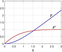
The condition for ${\displaystyle v_{z}}$ as ${\displaystyle z\rightarrow \infty }$ cannot be prescribed and is obtained as a part of the solution. The problem formulated here is a special case of Falkner-Skan boundary layer. The solution can be obtained from numerical integrations and is shown in the figure. The asymptotic behaviors for large ${\displaystyle \eta \rightarrow \infty }$ are

${\displaystyle F\sim \eta -0.6479,\quad v_{x}\sim kx,\quad v_{z}\sim -k(z-\delta ^{*}),\quad \delta ^{*}=0.6479\delta }$

where ${\displaystyle \delta ^{*}}$ is the displacement thickness.

Stagnation point flow with a translating wall

Hiemenz flow when the solid wall translates with a constant velocity ${\displaystyle U}$ along the ${\displaystyle x}$ was solved by Rott (1956). ^[10] This problem describes the flow in the neighbourhood of the forward stagnation line occurring in a flow over a rotating cylinder. ^[11] The required stream function is

${\displaystyle \psi ={\sqrt {\nu k}}xF(\eta )+U\delta \int _{0}^{\eta }G(\eta )d\eta }$

where the function ${\displaystyle G(\eta )}$ satisfies

${\displaystyle G''+FG'-F'G=0,\quad G(0)=1,\quad G(\infty )=0}$

The solution to the above equation is given by ${\displaystyle G(\eta )=F''(\eta )/F''(0).}$

Oblique stagnation point flow

If the incoming stream is perpendicular to the stagnation line, but approaches obliquely, the outer flow is not potential, but has a constant vorticity ${\displaystyle -\zeta _{o}}$. The appropriate stream function for oblique stagnation point flow is given by

${\displaystyle \psi =kxz+{\frac {1}{2}}\zeta _{o}z^{2}}$

Viscous effects due to the presence of a solid wall was studied by Stuart (1959), ^[12] Tamada (1979) ^[13] and Dorrepaal (1986). ^[14] In their approach, the streamfunction takes the form

${\displaystyle \psi ={\sqrt {\nu k}}xF(\eta )+\zeta _{o}\delta ^{2}\int _{0}^{\eta }H(\eta )d\eta }$

where the function ${\displaystyle H(\eta )}$

${\displaystyle H''+FH'-F'H=0,\quad H(0)=0,\quad H'(\infty )=1}$.

Homann flow

Homann flow with injection

Homann flow with suction

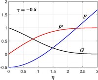
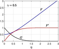
The solution for axisymmetric stagnation point flow in the presence of a solid wall was first obtained by Homann (1936). ^[15] A typical example of this flow is the forward stagnation point appearing in a flow past a sphere. Paul A. Libby (1974) ^[16] (1976) ^[17] extended Homann's work by allowing the solid wall to translate along its own plane with a constant speed and allowing constant suction or injection at the solid surface.

The solution for this problem is obtained in the cylindrical coordinate system ${\displaystyle (r,\theta ,z)}$ by introducing

${\displaystyle \eta ={\frac {z}{\sqrt {\nu /k}}},\quad \gamma =-{\frac {V}{2{\sqrt {k\nu }}}},\quad v_{r}=krF'(\eta )+U\cos \theta G(\eta ),\quad v_{\theta }=-U\sin \theta G(\eta ),\quad v_{z}=-2{\sqrt {k\nu }}F(\eta )}$

where ${\displaystyle U}$ is the translational speed of the wall and ${\displaystyle V}$ is the injection (or, suction) velocity at the wall. The problem is axisymmetric only when ${\displaystyle U=0}$. The pressure is given by

${\displaystyle {\frac {p-p_{o}}{\rho }}=-{\frac {1}{2}}k^{2}r^{2}-2k\nu (F^{2}+F')}$

The Navier–Stokes equations then reduce to

${\displaystyle {\begin{aligned}F'''+2FF''-F'^{2}+1&=0,\\G''+2FG'-F'G&=0\end{aligned}}}$

along with boundary conditions,

${\displaystyle F(0)=\gamma ,\quad F'(0)=0,\quad F'(\infty )=1,\quad G(0)=1,\quad G(\infty )=0.}$

When ${\displaystyle U=V=0}$, the classical Homann problem is recovered.

Plane counterflows

Jets emerging from a slot-jets creates stagnation point in between according to potential theory. The flow near the stagnation point can by studied using self-similar solution. This setup is widely used in combustion experiments. The initial study of impinging stagnation flows are due to C.Y. Wang. ^{[18] [19]} Let two fluids with constant properties denoted with suffix ${\displaystyle 1({\text{top}}),\ 2({\text{bottom}})}$ flowing from opposite direction impinge, and assume the two fluids are immiscible and the interface (located at ${\displaystyle y=0}$) is planar. The velocity is given by

${\displaystyle u_{1}=k_{1}x,\quad v_{1}=-k_{1}y,\quad u_{2}=k_{2}x,\quad v_{2}=-k_{2}y}$

where ${\displaystyle k_{1},\ k_{2}}$ are strain rates of the fluids. At the interface, velocities, tangential stress and pressure must be continuous. Introducing the self-similar transformation,

${\displaystyle \eta _{1}={\sqrt {\frac {\nu _{1}}{k_{1}}}}y,\quad u_{1}=k_{1}xF_{1}',\quad v_{1}=-{\sqrt {\nu _{1}k_{1}}}F_{1}}$

${\displaystyle \eta _{2}={\sqrt {\frac {\nu _{2}}{k_{2}}}}y,\quad u_{2}=k_{2}xF_{2}',\quad v_{2}=-{\sqrt {\nu _{2}k_{2}}}F_{2}}$

results equations,

${\displaystyle F_{1}'''+F_{1}F_{1}''-F_{1}'^{2}+1=0,\quad {\frac {p_{o1}-p_{1}}{\rho _{1}}}={\frac {1}{2}}k_{1}^{2}x^{2}+k_{1}\nu _{1}F_{1}'+{\frac {1}{2}}k_{1}\nu _{1}F_{1}^{2}}$

${\displaystyle F_{2}'''+F_{2}F_{2}''-F_{2}'^{2}+1=0,\quad {\frac {p_{o2}-p_{2}}{\rho _{2}}}={\frac {1}{2}}k_{2}^{2}x^{2}+k_{2}\nu _{2}F_{2}'+{\frac {1}{2}}k_{2}\nu _{2}F_{2}^{2}.}$

The no-penetration condition at the interface and free stream condition far away from the stagnation plane become

${\displaystyle F_{1}(0)=0,\quad F_{1}'(\infty )=1,\quad F_{2}(0)=0,\quad F_{2}'(-\infty )=1.}$

But the equations require two more boundary conditions. At ${\displaystyle \eta =0}$, the tangential velocities ${\displaystyle u_{1}=u_{2}}$, the tangential stress ${\displaystyle \rho _{1}\nu _{1}\partial u_{1}/\partial y=\rho _{2}\nu _{2}\partial u_{2}/\partial y}$ and the pressure ${\displaystyle p_{1}=p_{2}}$ are continuous. Therefore,

${\displaystyle {\begin{aligned}k_{1}F_{1}'(0)&=k_{2}F_{2}'(0),\\\rho _{1}{\sqrt {\nu _{1}k_{1}^{3}}}F_{1}''(0)&=\rho _{2}{\sqrt {\nu _{2}k_{2}^{3}}}F_{2}''(0),\\p_{o1}-\rho _{1}\nu _{1}k_{1}F_{1}'(0)&=p_{o2}-\rho _{2}\nu _{2}k_{2}F_{2}'(0).\end{aligned}}}$

where ${\displaystyle \rho _{1}k_{1}^{2}=\rho _{2}k_{2}^{2}}$ (from outer inviscid problem) is used. Both ${\displaystyle F_{i}'(0),F_{i}''(0)}$ are not known apriori, but derived from matching conditions. The third equation is determine variation of outer pressure ${\displaystyle p_{o1}-p_{o2}}$ due to the effect of viscosity. So there are only two parameters, which governs the flow, which are

${\displaystyle \Lambda ={\frac {k_{1}}{k_{2}}}=\left({\frac {\rho _{2}}{\rho _{1}}}\right)^{1/2},\quad \Gamma ={\frac {\nu _{2}}{\nu _{1}}}}$

then the boundary conditions become

${\displaystyle F_{1}'(0)=\Lambda F_{2}'(0),\quad F_{1}''(0)={\sqrt {\frac {\Gamma }{\Lambda }}}F_{2}''(0)}$.

References

1. Moffatt, H. K., Kida, S., & Ohkitani, K. (1994). Stretched vortices–the sinews of turbulence; large-Reynolds-number asymptotics. Journal of Fluid Mechanics, 259, 241-264.
2. Taylor, G. I. (1934). The formation of emulsions in definable fields of flow. Proceedings of the Royal Society of London. Series A, containing papers of a mathematical and physical character, 146(858), 501-523.
3. Wang, C. Y. (1974). Axisymmetric stagnation flow on a cylinder. Quarterly of Applied Mathematics, 32(2), 207-213.
4. Craik, A. D. (2009). Exact vortex solutions of the Navier–Stokes equations with axisymmetric strain and suction or injection. Journal of fluid mechanics, 626, 291-306.
5. Rajamanickam, P., & Weiss, A. D. (2021). Steady axisymmetric vortices in radial stagnation flows. The Quarterly Journal of Mechanics and Applied Mathematics, 74(3), 367-378.
6. Hiemenz, Karl (1911) "Die Grenzschicht an einem in den gleichförmigen Flüssigkeitsstrom eingetauchten geraden Kreiszylinder"
7. Howarth, Leslie (1934) On the calculation of steady flow in the boundary layer near the surface of a cylinder in a stream. No. ARC-R/M-1632. AERONAUTICAL RESEARCH COUNCIL LONDON (UNITED KINGDOM)
8. Rosenhead, Louis, editor (1963) Laminar boundary layers, Clarendon Press
9. Batchelor, George Keith (2000) An introduction to fluid dynamics, Cambridge University Press
10. Rott, Nicholas. "Unsteady viscous flow in the vicinity of a stagnation point." Quarterly of Applied Mathematics 13.4 (1956): 444–451.
11. Drazin, Philip G., and Norman Riley (2006) The Navier–Stokes equations: a classification of flows and exact solutions. No. 334. Cambridge University Press
12. J. T. Stuart (2012) "The viscous flow near a stagnation point when the external flow has uniform vorticity." Journal of the Aerospace Sciences
13. Tamada, Ko. "Two-dimensional stagnation-point flow impinging obliquely on a plane wall." Journal of the Physical Society of Japan 46 (1979): 310.
14. Dorrepaal, J. M. "An exact solution of the Navier–Stokes equation which describes non-orthogonal stagnation-point flow in two dimensions." Journal of Fluid Mechanics 163 (1986): 141–147.
15. Homann, Fritz. "Der Einfluss grosser Zähigkeit bei der Strömung um den Zylinder und um die Kugel." ZAMM‐Journal of Applied Mathematics and Mechanics/Zeitschrift für Angewandte Mathematik und Mechanik 16.3 (1936): 153–164.
16. Libby, Paul A. "Wall shear at a three-dimensional stagnation point with a moving wall." AIAA Journal 12.3 (1974): 408–409.
17. Libby, Paul A. "Laminar flow at a three-dimensional stagnation point with large rates of injection." AIAA Journal 14.9 (1976): 1273–1279.
18. Wang, C. Y. "Stagnation flow on the surface of a quiescent fluid—an exact solution of the Navier–Stokes equations." Quarterly of applied mathematics 43.2 (1985): 215–223.
19. Wang, C. Y. "Impinging stagnation flows." The Physics of fluids 30.3 (1987): 915–917.