Stein's unbiased risk estimate

Last updated December 15, 2020

In statistics, Stein's unbiased risk estimate (SURE) is an unbiased estimator of the mean-squared error of "a nearly arbitrary, nonlinear biased estimator."^[1] In other words, it provides an indication of the accuracy of a given estimator. This is important since the true mean-squared error of an estimator is a function of the unknown parameter to be estimated, and thus cannot be determined exactly.

Formal statement

Let $\mu \in {\mathbb {R} }^{d}$ be an unknown parameter and let $x\in {\mathbb {R} }^{d}$ be a measurement vector whose components are independent and distributed normally with mean $\mu _{i},i=1,...,d,$ and variance $\sigma ^{2}$ . Suppose $h(x)$ is an estimator of $\mu$ from $x$ , and can be written $h(x)=x+g(x)$ , where $g$ is weakly differentiable. Then, Stein's unbiased risk estimate is given by^[3]

\operatorname {SURE} (h)=d\sigma ^{2}+\|g(x)\|^{2}+2\sigma ^{2}\sum _{i=1}^{d}{\frac {\partial }{\partial x_{i}}}g_{i}(x)=-d\sigma ^{2}+\|g(x)\|^{2}+2\sigma ^{2}\sum _{i=1}^{d}{\frac {\partial }{\partial x_{i}}}h_{i}(x),

where $g_{i}(x)$ is the $i$ th component of the function $g(x)$ , and $\|\cdot \|$ is the Euclidean norm.

The importance of SURE is that it is an unbiased estimate of the mean-squared error (or squared error risk) of $h(x)$ , i.e.

\operatorname {E} _{\mu }\{\operatorname {SURE} (h)\}=\operatorname {MSE} (h),\,\!

with

\operatorname {MSE} (h)=\operatorname {E} _{\mu }\|h(x)-\mu \|^{2}.

Thus, minimizing SURE can act as a surrogate for minimizing the MSE. Note that there is no dependence on the unknown parameter $\mu$ in the expression for SURE above. Thus, it can be manipulated (e.g., to determine optimal estimation settings) without knowledge of $\mu$ .

Proof

We wish to show that

\operatorname {E} _{\mu }\|h(x)-\mu \|^{2}=\operatorname {E} _{\mu }\{\operatorname {SURE} (h)\}.

We start by expanding the MSE as

{\begin{aligned}\operatorname {E} _{\mu }\|h(x)-\mu \|^{2}&=\operatorname {E} _{\mu }\|g(x)+x-\mu \|^{2}\\&=\operatorname {E} _{\mu }\|g(x)\|^{2}+\operatorname {E} _{\mu }\|x-\mu \|^{2}+2\operatorname {E} _{\mu }g(x)^{T}(x-\mu )\\&=\operatorname {E} _{\mu }\|g(x)\|^{2}+d\sigma ^{2}+2\operatorname {E} _{\mu }g(x)^{T}(x-\mu ).\end{aligned}}

Now we use integration by parts to rewrite the last term:

{\begin{aligned}\operatorname {E} _{\mu }g(x)^{T}(x-\mu )&=\int _{{\mathbb {R} }^{d}}{\frac {1}{\sqrt {2\pi \sigma ^{2d}}}}\exp \left(-{\frac {\|x-\mu \|^{2}}{2\sigma ^{2}}}\right)\sum _{i=1}^{d}g_{i}(x)(x_{i}-\mu _{i})d^{d}x\\&=\sigma ^{2}\sum _{i=1}^{d}\int _{{\mathbb {R} }^{d}}{\frac {1}{\sqrt {2\pi \sigma ^{2d}}}}\exp \left(-{\frac {\|x-\mu \|^{2}}{2\sigma ^{2}}}\right){\frac {dg_{i}}{dx_{i}}}d^{d}x\\&=\sigma ^{2}\sum _{i=1}^{d}\operatorname {E} _{\mu }{\frac {dg_{i}}{dx_{i}}}.\end{aligned}}

Substituting this into the expression for the MSE, we arrive at

\operatorname {E} _{\mu }\|h(x)-\mu \|^{2}=\operatorname {E} _{\mu }\left(d\sigma ^{2}+\|g(x)\|^{2}+2\sigma ^{2}\sum _{i=1}^{d}{\frac {dg_{i}}{dx_{i}}}\right).

Applications

A standard application of SURE is to choose a parametric form for an estimator, and then optimize the values of the parameters to minimize the risk estimate. This technique has been applied in several settings. For example, a variant of the James–Stein estimator can be derived by finding the optimal shrinkage estimator.^[2] The technique has also been used by Donoho and Johnstone to determine the optimal shrinkage factor in a wavelet denoising setting.^[1]

Related Research Articles

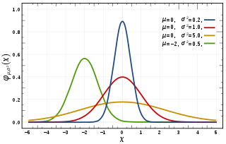
In probability theory, a normaldistribution is a type of continuous probability distribution for a real-valued random variable. The general form of its probability density function is

In probability theory and statistics, variance is the expectation of the squared deviation of a random variable from its mean. Informally, it measures how far a set of numbers is spread out from their average value. Variance has a central role in statistics, where some ideas that use it include descriptive statistics, statistical inference, hypothesis testing, goodness of fit, and Monte Carlo sampling. Variance is an important tool in the sciences, where statistical analysis of data is common. The variance is the square of the standard deviation, the second central moment of a distribution, and the covariance of the random variable with itself, and it is often represented by $,, or .$

The weighted arithmetic mean is similar to an ordinary arithmetic mean, except that instead of each of the data points contributing equally to the final average, some data points contribute more than others. The notion of weighted mean plays a role in descriptive statistics and also occurs in a more general form in several other areas of mathematics.

Multivariate normal distribution Generalization of the one-dimensional normal distribution to higher dimensions

In probability theory and statistics, the multivariate normal distribution, multivariate Gaussian distribution, or joint normal distribution is a generalization of the one-dimensional (univariate) normal distribution to higher dimensions. One definition is that a random vector is said to be k-variate normally distributed if every linear combination of its k components has a univariate normal distribution. Its importance derives mainly from the multivariate central limit theorem. The multivariate normal distribution is often used to describe, at least approximately, any set of (possibly) correlated real-valued random variables each of which clusters around a mean value.

In probability theory, a log-normal distribution is a continuous probability distribution of a random variable whose logarithm is normally distributed. Thus, if the random variable $X$ is log-normally distributed, then $Y = ln(X)$ has a normal distribution. Equivalently, if $Y$ has a normal distribution, then the exponential function of $Y$ , $X = exp(Y)$ , has a log-normal distribution. A random variable which is log-normally distributed takes only positive real values. It is a convenient and useful model for measurements in exact and engineering sciences, as well as medicine, economics and other topics.

In statistics, maximum likelihood estimation (MLE) is a method of estimating the parameters of a probability distribution by maximizing a likelihood function, so that under the assumed statistical model the observed data is most probable. The point in the parameter space that maximizes the likelihood function is called the maximum likelihood estimate. The logic of maximum likelihood is both intuitive and flexible, and as such the method has become a dominant means of statistical inference.

In statistics, the mean squared error (MSE) or mean squared deviation (MSD) of an estimator measures the average of the squares of the errors—that is, the average squared difference between the estimated values and the actual value. MSE is a risk function, corresponding to the expected value of the squared error loss. The fact that MSE is almost always strictly positive is because of randomness or because the estimator does not account for information that could produce a more accurate estimate.

In estimation theory and statistics, the Cramér–Rao bound (CRB) expresses a lower bound on the variance of unbiased estimators of a deterministic parameter, stating that the variance of any such estimator is at least as high as the inverse of the Fisher information. The result is named in honor of Harald Cramér and C. R. Rao, but has independently also been derived by Maurice Fréchet, Georges Darmois, as well as Alexander Aitken and Harold Silverstone.

In statistics, sometimes the covariance matrix of a multivariate random variable is not known but has to be estimated. Estimation of covariance matrices then deals with the question of how to approximate the actual covariance matrix on the basis of a sample from the multivariate distribution. Simple cases, where observations are complete, can be dealt with by using the sample covariance matrix. The sample covariance matrix (SCM) is an unbiased and efficient estimator of the covariance matrix if the space of covariance matrices is viewed as an extrinsic convex cone in R^p×p; however, measured using the intrinsic geometry of positive-definite matrices, the SCM is a biased and inefficient estimator. In addition, if the random variable has normal distribution, the sample covariance matrix has Wishart distribution and a slightly differently scaled version of it is the maximum likelihood estimate. Cases involving missing data require deeper considerations. Another issue is the robustness to outliers, to which sample covariance matrices are highly sensitive.

In statistics, a consistent estimator or asymptotically consistent estimator is an estimator—a rule for computing estimates of a parameter θ₀—having the property that as the number of data points used increases indefinitely, the resulting sequence of estimates converges in probability to θ₀. This means that the distributions of the estimates become more and more concentrated near the true value of the parameter being estimated, so that the probability of the estimator being arbitrarily close to θ₀ converges to one.

In Bayesian statistics, a maximum a posteriori probability (MAP) estimate is an estimate of an unknown quantity, that equals the mode of the posterior distribution. The MAP can be used to obtain a point estimate of an unobserved quantity on the basis of empirical data. It is closely related to the method of maximum likelihood (ML) estimation, but employs an augmented optimization objective which incorporates a prior distribution over the quantity one wants to estimate. MAP estimation can therefore be seen as a regularization of maximum likelihood estimation.

In estimation theory and decision theory, a Bayes estimator or a Bayes action is an estimator or decision rule that minimizes the posterior expected value of a loss function. Equivalently, it maximizes the posterior expectation of a utility function. An alternative way of formulating an estimator within Bayesian statistics is maximum a posteriori estimation.

Covariance matrix adaptation evolution strategy (CMA-ES) is a particular kind of strategy for numerical optimization. Evolution strategies (ES) are stochastic, derivative-free methods for numerical optimization of non-linear or non-convex continuous optimization problems. They belong to the class of evolutionary algorithms and evolutionary computation. An evolutionary algorithm is broadly based on the principle of biological evolution, namely the repeated interplay of variation and selection: in each generation (iteration) new individuals are generated by variation, usually in a stochastic way, of the current parental individuals. Then, some individuals are selected to become the parents in the next generation based on their fitness or objective function value $. Like this, over the generation sequence, individuals with better and better -values are generated.$

In statistics, the bias of an estimator is the difference between this estimator's expected value and the true value of the parameter being estimated. An estimator or decision rule with zero bias is called unbiased. In statistics, "bias" is an objective property of an estimator. Bias can also be measured with respect to the median, rather than the mean, in which case one distinguishes median-unbiased from the usual mean-unbiasedness property. Bias is a distinct concept from consistency. Consistent estimators converge in probability to the true value of the parameter, but may be biased or unbiased; see bias versus consistency for more.

In statistics, Bessel's correction is the use of n − 1 instead of n in the formula for the sample variance and sample standard deviation, where n is the number of observations in a sample. This method corrects the bias in the estimation of the population variance. It also partially corrects the bias in the estimation of the population standard deviation. However, the correction often increases the mean squared error in these estimations. This technique is named after Friedrich Bessel.

In credibility theory, a branch of study in actuarial science, the Bühlmann model is a random effects model used in to determine the appropriate premium for a group of insurance contracts. The model is named after Hans Bühlmann who first published a description in 1967.

In probability and statistics, the class of exponential dispersion models (EDM) is a set of probability distributions that represents a generalisation of the natural exponential family. Exponential dispersion models play an important role in statistical theory, in particular in generalized linear models because they have a special structure which enables deductions to be made about appropriate statistical inference.

In probability theory and directional statistics, a wrapped normal distribution is a wrapped probability distribution that results from the "wrapping" of the normal distribution around the unit circle. It finds application in the theory of Brownian motion and is a solution to the heat equation for periodic boundary conditions. It is closely approximated by the von Mises distribution, which, due to its mathematical simplicity and tractability, is the most commonly used distribution in directional statistics.

In the comparison of various statistical procedures, efficiency is a measure of quality of an estimator, of an experimental design, or of a hypothesis testing procedure. Essentially, a more efficient estimator, experiment, or test needs fewer observations than a less efficient one to achieve a given performance. This article primarily deals with efficiency of estimators.

In statistics, the variance function is a smooth function which depicts the variance of a random quantity as a function of its mean. The variance function plays a large role in many settings of statistical modelling. It is a main ingredient in the generalized linear model framework and a tool used in non-parametric regression, semiparametric regression and functional data analysis. In parametric modeling, variance functions take on a parametric form and explicitly describe the relationship between the variance and the mean of a random quantity. In a non-parametric setting, the variance function is assumed to be a smooth function.

References

1 2 Donoho, David L.; Iain M. Johnstone (December 1995). "Adapting to Unknown Smoothness via Wavelet Shrinkage". Journal of the American Statistical Association. 90 (432): 1200–1244. CiteSeerX 10.1.1.161.8697 . doi:10.2307/2291512. JSTOR 2291512.
1 2 Stein, Charles M. (November 1981). "Estimation of the Mean of a Multivariate Normal Distribution". The Annals of Statistics. 9 (6): 1135–1151. doi: 10.1214/aos/1176345632 . JSTOR 2240405.
↑ Wasserman, Larry (2005). All of Nonparametric Statistics.

This page is based on this Wikipedia article
Text is available under the CC BY-SA 4.0 license; additional terms may apply.
Images, videos and audio are available under their respective licenses.

[donoho95-1] 1 2 Donoho, David L.; Iain M. Johnstone (December 1995). "Adapting to Unknown Smoothness via Wavelet Shrinkage". Journal of the American Statistical Association. 90 (432): 1200–1244. CiteSeerX 10.1.1.161.8697 . doi:10.2307/2291512. JSTOR 2291512.

[stein81-2] 1 2 Stein, Charles M. (November 1981). "Estimation of the Mean of a Multivariate Normal Distribution". The Annals of Statistics. 9 (6): 1135–1151. doi: 10.1214/aos/1176345632 . JSTOR 2240405.

[wasserman05-3] Wasserman, Larry (2005). All of Nonparametric Statistics.

[1]

[2]

[3]