Tensor product model transformation

Last updated December 19, 2024

In mathematics, the tensor product (TP) model transformation was proposed by Baranyi and Yam^[1]^[2]^[3]^[4]^[5] as key concept for higher-order singular value decomposition of functions. It transforms a function (which can be given via closed formulas or neural networks, fuzzy logic, etc.) into TP function form if such a transformation is possible. If an exact transformation is not possible, then the method determines a TP function that is an approximation of the given function. Hence, the TP model transformation can provide a trade-off between approximation accuracy and complexity.^[6]

Besides being a transformation of functions, the TP model transformation is also a new concept in qLPV based control which plays a central role in the providing a valuable means of bridging between identification and polytopic systems theories. The TP model transformation is uniquely effective in manipulating the convex hull of polytopic forms, and, as a result has revealed and proved the fact that convex hull manipulation is a necessary and crucial step in achieving optimal solutions and decreasing conservativeness^[8]^[9]^[2] in modern LMI based control theory. Thus, although it is a transformation in a mathematical sense, it has established a conceptually new direction in control theory and has laid the ground for further new approaches towards optimality. Further details on the control theoretical aspects of the TP model transformation can be found here: TP model transformation in control theory.

The TP model transformation motivated the definition of the "HOSVD canonical form of TP functions",^[10] on which further information can be found here. It has been proved that the TP model transformation is capable of numerically reconstructing this HOSVD based canonical form.^[11] Thus, the TP model transformation can be viewed as a numerical method to compute the HOSVD of functions, which provides exact results if the given function has a TP function structure and approximative results otherwise.

The TP model transformation has recently been extended in order to derive various types of convex TP functions and to manipulate them.^[3] This feature has led to new optimization approaches in qLPV system analysis and design, as described at TP model transformation in control theory.

Definitions

Finite element TP function: A given function $f({\mathbf {x} })$ , where $\mathbf {x} \in R^{N}$ , is a TP function if it has the structure:

f(\mathbf {x} )=\sum _{i_{1}=1}^{I_{1}}\sum _{i_{2}=1}^{I_{2}}\ldots \sum _{i_{N}=1}^{I_{N}}\prod _{n=1}^{N}w_{n,i_{n}}(x_{n})s_{i_{1},i_{2},\ldots ,i_{N}},

that is, using compact tensor notation (using the tensor product operation $\otimes$ of ^[7] ):

f(\mathbf {x} )={\mathcal {S}}\mathop {\otimes } _{n=1}^{N}\mathbf {w} _{n}(x_{n}),

where core tensor ${\mathcal {S}}\in {\mathcal {R}}^{I_{1}\times I_{2}\times \ldots \times I_{N}}$ is constructed from $s_{i_{1}i_{2}\ldots i_{N}}$ , and row vector $\mathbf {w} _{n}(x_{n}),(n=1\ldots N)$ contains continuous univariate weighting functions $w_{n,i_{n}}(x_{n}),(i_{n}=1\ldots I_{n})$ . The function $w_{n,i_{n}}(x_{n})$ is the $i_{n}$ -th weighting function defined on the $n$ -th dimension, and $x_{n}$ is the $n$ -the element of vector $\mathbf {x}$ . Finite element means that $I_{n}$ is bounded for all $n$ . For qLPV modelling and control applications a higher structure of TP functions are referred to as TP model.

Finite element TP model (TP model in short): This is a higher structure of TP function:

{\mathcal {F}}(\mathbf {x} )={\mathcal {S}}\boxtimes _{n=1}^{N}\mathbf {w} _{n}(x_{n}).

Here ${\mathcal {Y}}={\mathcal {F}}({\mathbf {x} })$ is a tensor as ${\mathcal {Y}}\in {\mathcal {R}}^{L_{1}\times L_{2}\times \ldots L_{O}}$ , thus the size of the core tensor is ${\mathcal {S}}\in {\mathcal {R}}^{I_{1}\times I_{2}\times \ldots \times I_{N}\times L_{1}\times L_{2}\times ...\times L_{O}}$ . The product operator $\boxtimes$ has the same role as $\otimes$ , but expresses the fact that the tensor product is applied on the $L_{1}\times L_{2}\times ...\times L_{O}$ sized tensor elements of the core tensor ${\mathcal {S}}$ . Vector $\mathbf {x}$ is an element of the closed hypercube $\Omega =[a_{1},b_{1}]\times [a_{2},b_{2}]\times ...\times [a_{N},b_{N}]\subset R^{N}$ .

Finite element convex TP function or model: A TP function or model is convex if the weighting functions hold:

\forall n:\sum _{i_{n}=1}^{I_{n}}w_{n,i_{n}}(x_{n})=1

and

w_{n,i_{n}}(x_{n})\in [0,1].

This means that $f(\mathbf {x} )$ is inside the convex hull defined by the core tensor for all $\mathbf {x} \in \Omega$ .

TP model transformation: Assume a given TP model ${\mathcal {Y}}={\mathcal {F}}(\mathbf {x} )$ , where $\mathbf {x} \in \Omega \subset R^{N}$ , whose TP structure maybe unknown (e.g. it is given by neural networks). The TP model transformation determines its TP structure as

{\mathcal {F}}(\mathbf {x} )={\mathcal {S}}\boxtimes _{n=1}^{N}\mathbf {w} _{n}(x_{n})

,

namely it generates the core tensor ${\mathcal {S}}$ and the weighting functions $\mathbf {w} _{n}(x_{n})$ for all $n=1\ldots N$ . Its free MATLAB implementation is downloadable at or at MATLAB Central .

If the given ${\mathcal {F}}(\mathbf {x} )$ does not have TP structure (i.e. it is not in the class of TP models), then the TP model transformation determines its approximation:[6]

{\mathcal {F}}(\mathbf {x} )\approx {\mathcal {S}}\boxtimes _{n=1}^{N}\mathbf {w} _{n}(x_{n}),

where trade-off is offered by the TP model transformation between complexity (number of components in the core tensor or the number of weighting functions) and the approximation accuracy. The TP model can be generated according to various constrains. Typical TP models generated by the TP model transformation are:

HOSVD canonical form of TP functions or TP model (qLPV models),
Various kinds of TP type polytopic form or convex TP model forms (this advantage is used in qLPV system analysis and design).

Properties of the TP model transformation

It is a non-heuristic and tractable numerical method firstly proposed in control theory.^[1]^[4]
It transforms the given function into finite element TP structure. If this structure does not exist, then the transformation gives an approximation under a constraint on the number of elements.
It can be executed uniformly (irrespective of whether the model is given in the form of analytical equations resulting from physical considerations, or as an outcome of soft computing based identification techniques (such as neural networks or fuzzy logic based methods, or as a result of a black-box identification), without analytical interaction, within a reasonable amount of time. Thus, the transformation replaces the analytical and in many cases complex and not obvious conversions to numerical, tractable, straightforward operations.
It generates the HOSVD-based canonical form of TP functions,^[10] which is a unique representation. It was proven by Szeidl ^[11] that the TP model transformation numerically reconstructs the HOSVD of functions. This form extracts the unique structure of a given TP function in the same sense as the HOSVD does for tensors and matrices, in a way such that:

the number of weighting functions are minimized per dimensions (hence the size of the core tensor);
the weighting functions are one variable functions of the parameter vector in an orthonormed system for each parameter (singular functions);
the sub tensors of the core tensor are also in orthogonal positions;
the core tensor and the weighting functions are ordered according to the higher-order singular values of the parameter vector;
it has a unique form (except for some special cases such as there are equal singular values);
introduces and defines the rank of the TP function by the dimensions of the parameter vector;

The above point can be extended to TP models (qLPV models to determine the HOSVD based canonical form of qLPV model to order the main component of the qLPV model). Since the core tensor is $N+O$ dimensional, but the weighting functions are determined only for dimensions $n=1\ldots N$ , namely the core tensor is constructed from $O$ dimensional elements, therefore the resulting TP form is not unique.
The core step of the TP model transformation was extended to generate different types of convex TP functions or TP models (TP type polytopic qLPV models), in order to focus on the systematic (numerical and automatic) modification of the convex hull instead of developing new LMI equations for feasible controller design (this is the widely adopted approach). It is worth noting that both the TP model transformation and the LMI-based control design methods are numerically executable one after the other, and this makes the resolution of a wide class of problems possible in a straightforward and tractable, numerical way.
The TP model transformation is capable of performing trade-off between complexity and accuracy of TP functions ^[6] via discarding the higher-order singular values, in the same manner as the tensor HOSVD is used for complexity reduction.

Related Research Articles

Continuum mechanics is a branch of mechanics that deals with the deformation of and transmission of forces through materials modeled as a continuous medium rather than as discrete particles.

In mathematics, a normed vector space or normed space is a vector space over the real or complex numbers on which a norm is defined. A norm is a generalization of the intuitive notion of "length" in the physical world. If $is a vector space over, where is a field equal to or to, then a norm on is a map, typically denoted by, satisfying the following four axioms:$

Non-negativity: for every $, .$
Positive definiteness: for every $, if and only if is the zero vector.$
Absolute homogeneity: for every $and,$
Triangle inequality: for every $and,$

In mathematics, a product is the result of multiplication, or an expression that identifies objects to be multiplied, called factors. For example, 21 is the product of 3 and 7, and $is the product of and . When one factor is an integer, the product is called a multiple .$

In mathematics, a tensor is an algebraic object that describes a multilinear relationship between sets of algebraic objects related to a vector space. Tensors may map between different objects such as vectors, scalars, and even other tensors. There are many types of tensors, including scalars and vectors, dual vectors, multilinear maps between vector spaces, and even some operations such as the dot product. Tensors are defined independent of any basis, although they are often referred to by their components in a basis related to a particular coordinate system; those components form an array, which can be thought of as a high-dimensional matrix.

In Euclidean geometry, an affine transformation or affinity is a geometric transformation that preserves lines and parallelism, but not necessarily Euclidean distances and angles.

In mathematics, the $L p$ spaces are function spaces defined using a natural generalization of the $p$ -norm for finite-dimensional vector spaces. They are sometimes called Lebesgue spaces, named after Henri Lebesgue, although according to the Bourbaki group they were first introduced by Frigyes Riesz.

Noether's theorem states that every continuous symmetry of the action of a physical system with conservative forces has a corresponding conservation law. This is the first of two theorems published by mathematician Emmy Noether in 1918. The action of a physical system is the integral over time of a Lagrangian function, from which the system's behavior can be determined by the principle of least action. This theorem only applies to continuous and smooth symmetries of physical space.

Vapnik–Chervonenkis theory was developed during 1960–1990 by Vladimir Vapnik and Alexey Chervonenkis. The theory is a form of computational learning theory, which attempts to explain the learning process from a statistical point of view.

In functional analysis, it is often convenient to define a linear transformation on a complete, normed vector space $by first defining a linear transformation on a dense subset of and then continuously extending to the whole space via the theorem below. The resulting extension remains linear and bounded, and is thus continuous, which makes it a continuous linear extension .$

Convex optimization is a subfield of mathematical optimization that studies the problem of minimizing convex functions over convex sets. Many classes of convex optimization problems admit polynomial-time algorithms, whereas mathematical optimization is in general NP-hard.

In mathematics, nuclear spaces are topological vector spaces that can be viewed as a generalization of finite-dimensional Euclidean spaces and share many of their desirable properties. Nuclear spaces are however quite different from Hilbert spaces, another generalization of finite-dimensional Euclidean spaces. They were introduced by Alexander Grothendieck.

In machine learning, kernel machines are a class of algorithms for pattern analysis, whose best known member is the support-vector machine (SVM). These methods involve using linear classifiers to solve nonlinear problems. The general task of pattern analysis is to find and study general types of relations in datasets. For many algorithms that solve these tasks, the data in raw representation have to be explicitly transformed into feature vector representations via a user-specified feature map: in contrast, kernel methods require only a user-specified kernel, i.e., a similarity function over all pairs of data points computed using inner products. The feature map in kernel machines is infinite dimensional but only requires a finite dimensional matrix from user-input according to the Representer theorem. Kernel machines are slow to compute for datasets larger than a couple of thousand examples without parallel processing.

<span class="mw-page-title-main">Scoring rule</span> Measure for evaluating probabilistic forecasts

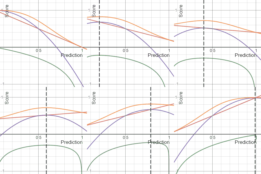
In decision theory, a scoring rule provides evaluation metrics for probabilistic predictions or forecasts. While "regular" loss functions assign a goodness-of-fit score to a predicted value and an observed value, scoring rules assign such a score to a predicted probability distribution and an observed value. On the other hand, a scoring function provides a summary measure for the evaluation of point predictions, i.e. one predicts a property or functional $, like the expectation or the median.$

In applied mathematics, polyharmonic splines are used for function approximation and data interpolation. They are very useful for interpolating and fitting scattered data in many dimensions. Special cases include thin plate splines and natural cubic splines in one dimension.

In multilinear algebra, the tensor rank decomposition or rank-R decomposition is the decomposition of a tensor as a sum of R rank-1 tensors, where R is minimal. Computing this decomposition is an open problem.

In multilinear algebra, the higher-order singular value decomposition (HOSVD) of a tensor is a specific orthogonal Tucker decomposition. It may be regarded as one type of generalization of the matrix singular value decomposition. It has applications in computer vision, computer graphics, machine learning, scientific computing, and signal processing. Some aspects can be traced as far back as F. L. Hitchcock in 1928, but it was L. R. Tucker who developed for third-order tensors the general Tucker decomposition in the 1960s, further advocated by L. De Lathauwer et al. in their Multilinear SVD work that employs the power method, or advocated by Vasilescu and Terzopoulos that developed M-mode SVD a parallel algorithm that employs the matrix SVD.

Within bayesian statistics for machine learning, kernel methods arise from the assumption of an inner product space or similarity structure on inputs. For some such methods, such as support vector machines (SVMs), the original formulation and its regularization were not Bayesian in nature. It is helpful to understand them from a Bayesian perspective. Because the kernels are not necessarily positive semidefinite, the underlying structure may not be inner product spaces, but instead more general reproducing kernel Hilbert spaces. In Bayesian probability kernel methods are a key component of Gaussian processes, where the kernel function is known as the covariance function. Kernel methods have traditionally been used in supervised learning problems where the input space is usually a space of vectors while the output space is a space of scalars. More recently these methods have been extended to problems that deal with multiple outputs such as in multi-task learning.

Baranyi and Yam proposed the TP model transformation as a new concept in quasi-LPV (qLPV) based control, which plays a central role in the highly desirable bridging between identification and polytopic systems theories. It is also used as a TS (Takagi-Sugeno) fuzzy model transformation. It is uniquely effective in manipulating the convex hull of polytopic forms, and, hence, has revealed and proved the fact that convex hull manipulation is a necessary and crucial step in achieving optimal solutions and decreasing conservativeness in modern linear matrix inequality based control theory. Thus, although it is a transformation in a mathematical sense, it has established a conceptually new direction in control theory and has laid the ground for further new approaches towards optimality.

Based on the key idea of higher-order singular value decomposition (HOSVD) in tensor algebra, Baranyi and Yam proposed the concept of HOSVD-based canonical form of TP functions and quasi-LPV system models. Szeidl et al. proved that the TP model transformation is capable of numerically reconstructing this canonical form.

Lagrangian field theory is a formalism in classical field theory. It is the field-theoretic analogue of Lagrangian mechanics. Lagrangian mechanics is used to analyze the motion of a system of discrete particles each with a finite number of degrees of freedom. Lagrangian field theory applies to continua and fields, which have an infinite number of degrees of freedom.

References

1 2 P. Baranyi (April 2004). "TP model transformation as a way to LMI based controller design". IEEE Transactions on Industrial Electronics. 51 (2): 387–400. doi:10.1109/tie.2003.822037. S2CID 7957799.
1 2 Baranyi, Péter (2016). TP-Model Transformation-Based-Control Design Frameworks. doi:10.1007/978-3-319-19605-3. ISBN 978-3-319-19604-6.
1 2 Baranyi, Peter (2014). "The Generalized TP Model Transformation for T–S Fuzzy Model Manipulation and Generalized Stability Verification". IEEE Transactions on Fuzzy Systems. 22 (4): 934–948. doi: 10.1109/TFUZZ.2013.2278982 .
1 2 P. Baranyi; D. Tikk; Y. Yam; R. J. Patton (2003). "From Differential Equations to PDC Controller Design via Numerical Transformation". Computers in Industry. 51 (3): 281–297. doi:10.1016/s0166-3615(03)00058-7.
↑ P. Baranyi; Y. Yam & P. Várlaki (2013). Tensor Product model transformation in polytopic model-based control. Boca Raton FL: Taylor & Francis. p. 240. ISBN 978-1-43-981816-9.
1 2 3 D. Tikk; P. Baranyi; R. J. Patton (2007). "Approximation Properties of TP Model Forms and its Consequences to TPDC Design Framework". Asian Journal of Control. 9 (3): 221–331. doi:10.1111/j.1934-6093.2007.tb00410.x. S2CID 121716136.
1 2 Lieven De Lathauwer; Bart De Moor; Joos Vandewalle (2000). "A Multilinear Singular Value Decomposition". SIAM Journal on Matrix Analysis and Applications. 21 (4): 1253–1278. CiteSeerX 10.1.1.3.4043 . doi:10.1137/s0895479896305696.
↑ A.Szollosi, and Baranyi, P. (2016). Influence of the Tensor Product model representation of qLPV models on the feasibility of Linear Matrix Inequality. Asian Journal of Control, 18(4), 1328-1342
↑ A. Szöllősi and P. Baranyi: „Improved control performance of the 3‐DoF aeroelastic wing section: a TP model based 2D parametric control performance optimization.” in Asian Journal of Control, 19(2), 450-466. / 2017
1 2 P. Baranyi; L. Szeidl; P. Várlaki; Y. Yam (July 3–5, 2006). Definition of the HOSVD-based canonical form of polytopic dynamic models. 3rd International Conference on Mechatronics (ICM 2006). Budapest, Hungary. pp. 660–665.
1 2 L. Szeidl & P. Várlaki (2009). "HOSVD Based Canonical Form for Polytopic Models of Dynamic Systems". Journal of Advanced Computational Intelligence and Intelligent Informatics. 13 (1): 52–60. doi: 10.20965/jaciii.2009.p0052 .

Baranyi, P. (2018). Extension of the Multi-TP Model Transformation to Functions with Different Numbers of Variables. Complexity, 2018.

External links

TPtoolBoxMATLAB

This page is based on this Wikipedia article
Text is available under the CC BY-SA 4.0 license; additional terms may apply.
Images, videos and audio are available under their respective licenses.

[Baranyi04-1] 1 2 P. Baranyi (April 2004). "TP model transformation as a way to LMI based controller design". IEEE Transactions on Industrial Electronics. 51 (2): 387–400. doi:10.1109/tie.2003.822037. S2CID 7957799.

[springer.com-2] 1 2 Baranyi, Péter (2016). TP-Model Transformation-Based-Control Design Frameworks. doi:10.1007/978-3-319-19605-3. ISBN 978-3-319-19604-6.

[P._Baranyi_2014,_pp._934-948-3] 1 2 Baranyi, Peter (2014). "The Generalized TP Model Transformation for T–S Fuzzy Model Manipulation and Generalized Stability Verification". IEEE Transactions on Fuzzy Systems. 22 (4): 934–948. doi: 10.1109/TFUZZ.2013.2278982 .

[compind-4] 1 2 P. Baranyi; D. Tikk; Y. Yam; R. J. Patton (2003). "From Differential Equations to PDC Controller Design via Numerical Transformation". Computers in Industry. 51 (3): 281–297. doi:10.1016/s0166-3615(03)00058-7.

[ykc00-5] P. Baranyi; Y. Yam & P. Várlaki (2013). Tensor Product model transformation in polytopic model-based control. Boca Raton FL: Taylor & Francis. p. 240. ISBN 978-1-43-981816-9.

[ykc01-6] 1 2 3 D. Tikk; P. Baranyi; R. J. Patton (2007). "Approximation Properties of TP Model Forms and its Consequences to TPDC Design Framework". Asian Journal of Control. 9 (3): 221–331. doi:10.1111/j.1934-6093.2007.tb00410.x. S2CID 121716136.

[Lath00-7] 1 2 Lieven De Lathauwer; Bart De Moor; Joos Vandewalle (2000). "A Multilinear Singular Value Decomposition". SIAM Journal on Matrix Analysis and Applications. 21 (4): 1253–1278. CiteSeerX 10.1.1.3.4043 . doi:10.1137/s0895479896305696.

[8] A.Szollosi, and Baranyi, P. (2016). Influence of the Tensor Product model representation of qLPV models on the feasibility of Linear Matrix Inequality. Asian Journal of Control, 18(4), 1328-1342

[9] A. Szöllősi and P. Baranyi: „Improved control performance of the 3‐DoF aeroelastic wing section: a TP model based 2D parametric control performance optimization.” in Asian Journal of Control, 19(2), 450-466. / 2017

[canon1-10] 1 2 P. Baranyi; L. Szeidl; P. Várlaki; Y. Yam (July 3–5, 2006). Definition of the HOSVD-based canonical form of polytopic dynamic models. 3rd International Conference on Mechatronics (ICM 2006). Budapest, Hungary. pp. 660–665.

[canon3-11] 1 2 L. Szeidl & P. Várlaki (2009). "HOSVD Based Canonical Form for Polytopic Models of Dynamic Systems". Journal of Advanced Computational Intelligence and Intelligent Informatics. 13 (1): 52–60. doi: 10.20965/jaciii.2009.p0052 .

[1]

[2]

[3]

[4]

[5]

[6]

[7]

[8]

[9]

[10]

[11]