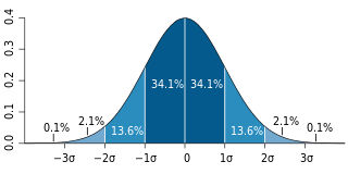
In statistics, the standard deviation is a measure of the amount of variation of the values of a variable about its mean. A low standard deviation indicates that the values tend to be close to the mean of the set, while a high standard deviation indicates that the values are spread out over a wider range. The standard deviation is commonly used in the determination of what constitutes an outlier and what does not.

In probability theory and statistics, variance is the expected value of the squared deviation from the mean of a random variable. The standard deviation (SD) is obtained as the square root of the variance. Variance is a measure of dispersion, meaning it is a measure of how far a set of numbers is spread out from their average value. It is the second central moment of a distribution, and the covariance of the random variable with itself, and it is often represented by , , , , or .

The Allan variance (AVAR), also known as two-sample variance, is a measure of frequency stability in clocks, oscillators and amplifiers. It is named after David W. Allan and expressed mathematically as . The Allan deviation (ADEV), also known as sigma-tau, is the square root of the Allan variance, .
In probability theory, Chebyshev's inequality provides an upper bound on the probability of deviation of a random variable from its mean. More specifically, the probability that a random variable deviates from its mean by more than is at most , where is any positive constant and is the standard deviation.
In statistical inference, specifically predictive inference, a prediction interval is an estimate of an interval in which a future observation will fall, with a certain probability, given what has already been observed. Prediction intervals are often used in regression analysis.
In statistics, propagation of uncertainty is the effect of variables' uncertainties on the uncertainty of a function based on them. When the variables are the values of experimental measurements they have uncertainties due to measurement limitations which propagate due to the combination of variables in the function.
In probability theory and statistics, a scale parameter is a special kind of numerical parameter of a parametric family of probability distributions. The larger the scale parameter, the more spread out the distribution.

In statistical modeling, regression analysis is a set of statistical processes for estimating the relationships between a dependent variable and one or more error-free independent variables. The most common form of regression analysis is linear regression, in which one finds the line that most closely fits the data according to a specific mathematical criterion. For example, the method of ordinary least squares computes the unique line that minimizes the sum of squared differences between the true data and that line. For specific mathematical reasons, this allows the researcher to estimate the conditional expectation of the dependent variable when the independent variables take on a given set of values. Less common forms of regression use slightly different procedures to estimate alternative location parameters or estimate the conditional expectation across a broader collection of non-linear models.
Ridge regression is a method of estimating the coefficients of multiple-regression models in scenarios where the independent variables are highly correlated. It has been used in many fields including econometrics, chemistry, and engineering. Also known as Tikhonov regularization, named for Andrey Tikhonov, it is a method of regularization of ill-posed problems. It is particularly useful to mitigate the problem of multicollinearity in linear regression, which commonly occurs in models with large numbers of parameters. In general, the method provides improved efficiency in parameter estimation problems in exchange for a tolerable amount of bias.

In statistics, ordinary least squares (OLS) is a type of linear least squares method for choosing the unknown parameters in a linear regression model by the principle of least squares: minimizing the sum of the squares of the differences between the observed dependent variable in the input dataset and the output of the (linear) function of the independent variable. Some sources consider OLS to be linear regression.
Exponential smoothing or exponential moving average (EMA) is a rule of thumb technique for smoothing time series data using the exponential window function. Whereas in the simple moving average the past observations are weighted equally, exponential functions are used to assign exponentially decreasing weights over time. It is an easily learned and easily applied procedure for making some determination based on prior assumptions by the user, such as seasonality. Exponential smoothing is often used for analysis of time-series data.
Weighted least squares (WLS), also known as weighted linear regression, is a generalization of ordinary least squares and linear regression in which knowledge of the unequal variance of observations (heteroscedasticity) is incorporated into the regression. WLS is also a specialization of generalized least squares, when all the off-diagonal entries of the covariance matrix of the errors, are null.

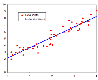
In statistics, simple linear regression (SLR) is a linear regression model with a single explanatory variable. That is, it concerns two-dimensional sample points with one independent variable and one dependent variable and finds a linear function that, as accurately as possible, predicts the dependent variable values as a function of the independent variable. The adjective simple refers to the fact that the outcome variable is related to a single predictor.
In statistics and in particular statistical theory, unbiased estimation of a standard deviation is the calculation from a statistical sample of an estimated value of the standard deviation of a population of values, in such a way that the expected value of the calculation equals the true value. Except in some important situations, outlined later, the task has little relevance to applications of statistics since its need is avoided by standard procedures, such as the use of significance tests and confidence intervals, or by using Bayesian analysis.
An alpha beta filter is a simplified form of observer for estimation, data smoothing and control applications. It is closely related to Kalman filters and to linear state observers used in control theory. Its principal advantage is that it does not require a detailed system model.
Demand forecasting, also known as demand planning and sales forecasting (DP&SF), involves the prediction of the quantity of goods and services that will be demanded by consumers or business customers at a future point in time. More specifically, the methods of demand forecasting entail using predictive analytics to estimate customer demand in consideration of key economic conditions. This is an important tool in optimizing business profitability through efficient supply chain management. Demand forecasting methods are divided into two major categories, qualitative and quantitative methods:
Experimental uncertainty analysis is a technique that analyses a derived quantity, based on the uncertainties in the experimentally measured quantities that are used in some form of mathematical relationship ("model") to calculate that derived quantity. The model used to convert the measurements into the derived quantity is usually based on fundamental principles of a science or engineering discipline.

In statistics, errors-in-variables models or measurement error models are regression models that account for measurement errors in the independent variables. In contrast, standard regression models assume that those regressors have been measured exactly, or observed without error; as such, those models account only for errors in the dependent variables, or responses.
In statistics, linear regression is a model that estimates the linear relationship between a scalar response and one or more explanatory variables. A model with exactly one explanatory variable is a simple linear regression; a model with two or more explanatory variables is a multiple linear regression. This term is distinct from multivariate linear regression, which predicts multiple correlated dependent variables rather than a single dependent variable.
Non-homogeneous Gaussian regression (NGR) is a type of statistical regression analysis used in the atmospheric sciences as a way to convert ensemble forecasts into probabilistic forecasts. Relative to simple linear regression, NGR uses the ensemble spread as an additional predictor, which is used to improve the prediction of uncertainty and allows the predicted uncertainty to vary from case to case. The prediction of uncertainty in NGR is derived from both past forecast errors statistics and the ensemble spread. NGR was originally developed for site-specific medium range temperature forecasting, but has since also been applied to site-specific medium-range wind forecasting and to seasonal forecasts, and has been adapted for precipitation forecasting. The introduction of NGR was the first demonstration that probabilistic forecasts that take account of the varying ensemble spread could achieve better skill scores than forecasts based on standard model output statistics approaches applied to the ensemble mean.


