
Probability theory or probability calculus is the branch of mathematics concerned with probability. Although there are several different probability interpretations, probability theory treats the concept in a rigorous mathematical manner by expressing it through a set of axioms. Typically these axioms formalise probability in terms of a probability space, which assigns a measure taking values between 0 and 1, termed the probability measure, to a set of outcomes called the sample space. Any specified subset of the sample space is called an event.
In probability theory and statistics, a probability distribution is the mathematical function that gives the probabilities of occurrence of different possible outcomes for an experiment. It is a mathematical description of a random phenomenon in terms of its sample space and the probabilities of events.
A random variable is a mathematical formalization of a quantity or object which depends on random events. The term 'random variable' can be misleading as it is not actually random nor a variable, but rather it is a function from possible outcomes in a sample space to a measurable space, often to the real numbers.
In probability theory, a probability space or a probability triple is a mathematical construct that provides a formal model of a random process or "experiment". For example, one can define a probability space which models the throwing of a die.
In probability theory, there exist several different notions of convergence of random variables. The convergence of sequences of random variables to some limit random variable is an important concept in probability theory, and its applications to statistics and stochastic processes. The same concepts are known in more general mathematics as stochastic convergence and they formalize the idea that a sequence of essentially random or unpredictable events can sometimes be expected to settle down into a behavior that is essentially unchanging when items far enough into the sequence are studied. The different possible notions of convergence relate to how such a behavior can be characterized: two readily understood behaviors are that the sequence eventually takes a constant value, and that values in the sequence continue to change but can be described by an unchanging probability distribution.
In mathematics, a degenerate distribution is, according to some, a probability distribution in a space with support only on a manifold of lower dimension, and according to others a distribution with support only at a single point. By the latter definition, it is a deterministic distribution and takes only a single value. Examples include a two-headed coin and rolling a die whose sides all show the same number. This distribution satisfies the definition of "random variable" even though it does not appear random in the everyday sense of the word; hence it is considered degenerate.
In probability and statistics, a Bernoulli process is a finite or infinite sequence of binary random variables, so it is a discrete-time stochastic process that takes only two values, canonically 0 and 1. The component Bernoulli variablesXi are identically distributed and independent. Prosaically, a Bernoulli process is a repeated coin flipping, possibly with an unfair coin. Every variable Xi in the sequence is associated with a Bernoulli trial or experiment. They all have the same Bernoulli distribution. Much of what can be said about the Bernoulli process can also be generalized to more than two outcomes ; this generalization is known as the Bernoulli scheme.

In probability and statistics, a probability mass function is a function that gives the probability that a discrete random variable is exactly equal to some value. Sometimes it is also known as the discrete probability density function. The probability mass function is often the primary means of defining a discrete probability distribution, and such functions exist for either scalar or multivariate random variables whose domain is discrete.

In probability theory, the law of large numbers (LLN) is a theorem that describes the result of performing the same experiment a large number of times. According to the law, the average of the results obtained from a large number of trials should be close to the expected value and tends to become closer to the expected value as more trials are performed.

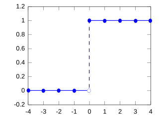
In probability theory and statistics, the Bernoulli distribution, named after Swiss mathematician Jacob Bernoulli, is the discrete probability distribution of a random variable which takes the value 1 with probability and the value 0 with probability . Less formally, it can be thought of as a model for the set of possible outcomes of any single experiment that asks a yes–no question. Such questions lead to outcomes that are boolean-valued: a single bit whose value is success/yes/true/one with probability p and failure/no/false/zero with probability q. It can be used to represent a coin toss where 1 and 0 would represent "heads" and "tails", respectively, and p would be the probability of the coin landing on heads. In particular, unfair coins would have
In probability theory and statistics, given two jointly distributed random variables and , the conditional probability distribution of given is the probability distribution of when is known to be a particular value; in some cases the conditional probabilities may be expressed as functions containing the unspecified value of as a parameter. When both and are categorical variables, a conditional probability table is typically used to represent the conditional probability. The conditional distribution contrasts with the marginal distribution of a random variable, which is its distribution without reference to the value of the other variable.
In information theory, the information content, self-information, surprisal, or Shannon information is a basic quantity derived from the probability of a particular event occurring from a random variable. It can be thought of as an alternative way of expressing probability, much like odds or log-odds, but which has particular mathematical advantages in the setting of information theory.
A continuous-time Markov chain (CTMC) is a continuous stochastic process in which, for each state, the process will change state according to an exponential random variable and then move to a different state as specified by the probabilities of a stochastic matrix. An equivalent formulation describes the process as changing state according to the least value of a set of exponential random variables, one for each possible state it can move to, with the parameters determined by the current state.
Probability theory and statistics have some commonly used conventions, in addition to standard mathematical notation and mathematical symbols.
In mathematics, the Gibbs measure, named after Josiah Willard Gibbs, is a probability measure frequently seen in many problems of probability theory and statistical mechanics. It is a generalization of the canonical ensemble to infinite systems. The canonical ensemble gives the probability of the system X being in state x as
In probability theory, random element is a generalization of the concept of random variable to more complicated spaces than the simple real line. The concept was introduced by Maurice Fréchet (1948) who commented that the “development of probability theory and expansion of area of its applications have led to necessity to pass from schemes where (random) outcomes of experiments can be described by number or a finite set of numbers, to schemes where outcomes of experiments represent, for example, vectors, functions, processes, fields, series, transformations, and also sets or collections of sets.”
In probability theory and statistical mechanics, the Gaussian free field (GFF) is a Gaussian random field, a central model of random surfaces (random height functions). Sheffield (2007) gives a mathematical survey of the Gaussian free field.

In probability theory and statistics, Fisher's noncentral hypergeometric distribution is a generalization of the hypergeometric distribution where sampling probabilities are modified by weight factors. It can also be defined as the conditional distribution of two or more binomially distributed variables dependent upon their fixed sum.
In mathematics – specifically, in the theory of stochastic processes – Doob's martingale convergence theorems are a collection of results on the limits of supermartingales, named after the American mathematician Joseph L. Doob. Informally, the martingale convergence theorem typically refers to the result that any supermartingale satisfying a certain boundedness condition must converge. One may think of supermartingales as the random variable analogues of non-increasing sequences; from this perspective, the martingale convergence theorem is a random variable analogue of the monotone convergence theorem, which states that any bounded monotone sequence converges. There are symmetric results for submartingales, which are analogous to non-decreasing sequences.
This article is supplemental for “Convergence of random variables” and provides proofs for selected results.


