Gaussian function

"Gaussian curve" redirects here. For the band, see Gaussian Curve (band).

In mathematics, a Gaussian function, often simply referred to as a Gaussian, is a function of the base form

$${\displaystyle f(x)=\exp(-x^{2})}$$

and with parametric extension

$${\displaystyle f(x)=a\exp \left(-{\frac {(x-b)^{2}}{2c^{2}}}\right)}$$

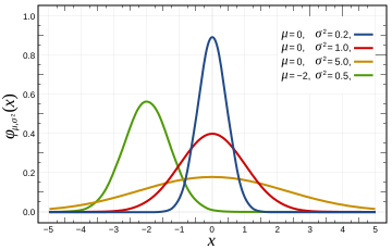
for arbitrary real constants a, b and non-zero c. It is named after the mathematician Carl Friedrich Gauss. The graph of a Gaussian is a characteristic symmetric "bell curve" shape. The parameter a is the height of the curve's peak, b is the position of the center of the peak, and c (the standard deviation, sometimes called the Gaussian RMS width) controls the width of the "bell".

Gaussian functions are often used to represent the probability density function of a normally distributed random variable with expected value μ = b and variance σ² = c². In this case, the Gaussian is of the form ^[1]

$${\displaystyle g(x)={\frac {1}{\sigma {\sqrt {2\pi }}}}\exp \left(-{\frac {1}{2}}{\frac {(x-\mu )^{2}}{\sigma ^{2}}}\right).}$$

Gaussian functions are widely used in statistics to describe the normal distributions, in signal processing to define Gaussian filters, in image processing where two-dimensional Gaussians are used for Gaussian blurs, and in mathematics to solve heat equations and diffusion equations and to define the Weierstrass transform.

Properties

Gaussian functions arise by composing the exponential function with a concave quadratic function:

$${\displaystyle f(x)=\exp(\alpha x^{2}+\beta x+\gamma ),}$$

where

• ${\displaystyle \alpha =-1/2c^{2},}$
• ${\displaystyle \beta =b/c^{2},}$
• ${\displaystyle \gamma =\ln a-(b^{2}/2c^{2}).}$

(Note: in ${\displaystyle \ln a,a=1/(\sigma {\sqrt {2\pi }})}$, not to be confused with ${\displaystyle \alpha =-1/2c^{2},}$)

The Gaussian functions are thus those functions whose logarithm is a concave quadratic function.

The parameter c is related to the full width at half maximum (FWHM) of the peak according to

$${\displaystyle {\text{FWHM}}=2{\sqrt {2\ln 2}}\,c\approx 2.35482\,c.}$$

The function may then be expressed in terms of the FWHM, represented by w:

$${\displaystyle f(x)=ae^{-4(\ln 2)(x-b)^{2}/w^{2}}.}$$

Alternatively, the parameter c can be interpreted by saying that the two inflection points of the function occur at x = b ± c.

The full width at tenth of maximum (FWTM) for a Gaussian could be of interest and is

$${\displaystyle {\text{FWTM}}=2{\sqrt {2\ln 10}}\,c\approx 4.29193\,c.}$$

Gaussian functions are analytic, and their limit as x → ∞ is 0 (for the above case of b = 0).

Gaussian functions are among those functions that are elementary but lack elementary antiderivatives; the integral of the Gaussian function is the error function:

$${\displaystyle \int e^{-x^{2}}\,dx={\frac {\sqrt {\pi }}{2}}\operatorname {erf} x+C.}$$

Nonetheless, their improper integrals over the whole real line can be evaluated exactly, using the Gaussian integral

$${\displaystyle \int _{-\infty }^{\infty }e^{-x^{2}}\,dx={\sqrt {\pi }},}$$

and one obtains

$${\displaystyle \int _{-\infty }^{\infty }ae^{-(x-b)^{2}/(2c^{2})}\,dx=ac\cdot {\sqrt {2\pi }}.}$$

Normalized Gaussian curves with expected value μ and variance σ. The corresponding parameters are ${\textstyle a={\tfrac {1}{\sigma {\sqrt {2\pi }}}}}$, b = μ and c = σ.

This integral is 1 if and only if ${\textstyle a={\tfrac {1}{c{\sqrt {2\pi }}}}}$ (the normalizing constant), and in this case the Gaussian is the probability density function of a normally distributed random variable with expected value μ = b and variance σ² = c²:

$${\displaystyle g(x)={\frac {1}{\sigma {\sqrt {2\pi }}}}\exp \left({\frac {-(x-\mu )^{2}}{2\sigma ^{2}}}\right).}$$

These Gaussians are plotted in the accompanying figure.

Gaussian functions centered at zero minimize the Fourier uncertainty principle ^{[ clarification needed ]}.

The product of two Gaussian functions is a Gaussian, and the convolution of two Gaussian functions is also a Gaussian, with variance being the sum of the original variances: ${\displaystyle c^{2}=c_{1}^{2}+c_{2}^{2}}$. The product of two Gaussian probability density functions (PDFs), though, is not in general a Gaussian PDF.

Taking the Fourier transform (unitary, angular-frequency convention) of a Gaussian function with parameters a = 1, b = 0 and c yields another Gaussian function, with parameters ${\displaystyle c}$, b = 0 and ${\displaystyle 1/c}$. ^[2] So in particular the Gaussian functions with b = 0 and ${\displaystyle c=1}$ are kept fixed by the Fourier transform (they are eigenfunctions of the Fourier transform with eigenvalue 1). A physical realization is that of the diffraction pattern: for example, a photographic slide whose transmittance has a Gaussian variation is also a Gaussian function.

The fact that the Gaussian function is an eigenfunction of the continuous Fourier transform allows us to derive the following interesting^{[ clarification needed ]} identity from the Poisson summation formula:

$${\displaystyle \sum _{k\in \mathbb {Z} }\exp \left(-\pi \cdot \left({\frac {k}{c}}\right)^{2}\right)=c\cdot \sum _{k\in \mathbb {Z} }\exp \left(-\pi \cdot (kc)^{2}\right).}$$

Integral of a Gaussian function

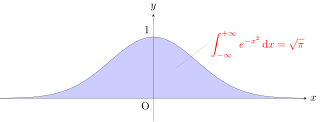
The integral of an arbitrary Gaussian function is

$${\displaystyle \int _{-\infty }^{\infty }a\,e^{-(x-b)^{2}/2c^{2}}\,dx={\sqrt {2}}a\,|c|\,{\sqrt {\pi }}.}$$

An alternative form is

$${\displaystyle \int _{-\infty }^{\infty }k\,e^{-fx^{2}+gx+h}\,dx=\int _{-\infty }^{\infty }k\,e^{-f{\big (}x-g/(2f){\big )}^{2}+g^{2}/(4f)+h}\,dx=k\,{\sqrt {\frac {\pi }{f}}}\,\exp \left({\frac {g^{2}}{4f}}+h\right),}$$

where f must be strictly positive for the integral to converge.

Relation to standard Gaussian integral

The integral

$${\displaystyle \int _{-\infty }^{\infty }ae^{-(x-b)^{2}/2c^{2}}\,dx}$$

for some real constants a, b, c > 0 can be calculated by putting it into the form of a Gaussian integral. First, the constant a can simply be factored out of the integral. Next, the variable of integration is changed from x to y = x − b:

$${\displaystyle a\int _{-\infty }^{\infty }e^{-y^{2}/2c^{2}}\,dy,}$$

and then to ${\displaystyle z=y/{\sqrt {2c^{2}}}}$:

$${\displaystyle a{\sqrt {2c^{2}}}\int _{-\infty }^{\infty }e^{-z^{2}}\,dz.}$$

Then, using the Gaussian integral identity

$${\displaystyle \int _{-\infty }^{\infty }e^{-z^{2}}\,dz={\sqrt {\pi }},}$$

we have

$${\displaystyle \int _{-\infty }^{\infty }ae^{-(x-b)^{2}/2c^{2}}\,dx=a{\sqrt {2\pi c^{2}}}.}$$

Two-dimensional Gaussian function

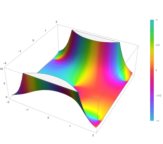
3d plot of a Gaussian function with a two-dimensional domain

Base form:

$${\displaystyle f(x,y)=\exp(-x^{2}-y^{2})}$$

In two dimensions, the power to which e is raised in the Gaussian function is any negative-definite quadratic form. Consequently, the level sets of the Gaussian will always be ellipses.

A particular example of a two-dimensional Gaussian function is

$${\displaystyle f(x,y)=A\exp \left(-\left({\frac {(x-x_{0})^{2}}{2\sigma _{X}^{2}}}+{\frac {(y-y_{0})^{2}}{2\sigma _{Y}^{2}}}\right)\right).}$$

Here the coefficient A is the amplitude, x₀, y₀ is the center, and σ_x, σ_y are the x and y spreads of the blob. The figure on the right was created using A = 1, x₀ = 0, y₀ = 0, σ_x = σ_y = 1.

The volume under the Gaussian function is given by

$${\displaystyle V=\int _{-\infty }^{\infty }\int _{-\infty }^{\infty }f(x,y)\,dx\,dy=2\pi A\sigma _{X}\sigma _{Y}.}$$

In general, a two-dimensional elliptical Gaussian function is expressed as

$${\displaystyle f(x,y)=A\exp {\Big (}-{\big (}a(x-x_{0})^{2}+2b(x-x_{0})(y-y_{0})+c(y-y_{0})^{2}{\big )}{\Big )},}$$

where the matrix

$${\displaystyle {\begin{bmatrix}a&b\\b&c\end{bmatrix}}}$$

is positive-definite.

Using this formulation, the figure on the right can be created using A = 1, (x₀, y₀) = (0, 0), a = c = 1/2, b = 0.

Meaning of parameters for the general equation

For the general form of the equation the coefficient A is the height of the peak and (x₀, y₀) is the center of the blob.

If we set

$${\displaystyle {\begin{aligned}a&={\frac {\cos ^{2}\theta }{2\sigma _{X}^{2}}}+{\frac {\sin ^{2}\theta }{2\sigma _{Y}^{2}}},\\b&=-{\frac {\sin \theta \cos \theta }{2\sigma _{X}^{2}}}+{\frac {\sin \theta \cos \theta }{2\sigma _{Y}^{2}}},\\c&={\frac {\sin ^{2}\theta }{2\sigma _{X}^{2}}}+{\frac {\cos ^{2}\theta }{2\sigma _{Y}^{2}}},\end{aligned}}}$$

then we rotate the blob by a positive, counter-clockwise angle ${\displaystyle \theta }$ (for negative, clockwise rotation, invert the signs in the b coefficient). ^[3]

To get back the coefficients ${\displaystyle \theta }$, ${\displaystyle \sigma _{X}}$ and ${\displaystyle \sigma _{Y}}$ from ${\displaystyle a}$, ${\displaystyle b}$ and ${\displaystyle c}$ use

${\displaystyle {\begin{aligned}\theta &={\frac {1}{2}}\arctan \left({\frac {2b}{a-c}}\right),\quad \theta \in [-45,45],\\\sigma _{X}^{2}&={\frac {1}{2(a\cdot \cos ^{2}\theta +2b\cdot \cos \theta \sin \theta +c\cdot \sin ^{2}\theta )}},\\\sigma _{Y}^{2}&={\frac {1}{2(a\cdot \sin ^{2}\theta -2b\cdot \cos \theta \sin \theta +c\cdot \cos ^{2}\theta )}}.\end{aligned}}}$

Example rotations of Gaussian blobs can be seen in the following examples:

${\displaystyle \theta =0}$

${\displaystyle \theta =-\pi /6}$

${\displaystyle \theta =-\pi /3}$

Using the following Octave code, one can easily see the effect of changing the parameters:

A=1;x0=0;y0=0;sigma_X=1;sigma_Y=2;[X,Y]=meshgrid(-5:.1:5,-5:.1:5);fortheta=0:pi/100:pia=cos(theta)^2/(2*sigma_X^2)+sin(theta)^2/(2*sigma_Y^2);b=sin(2*theta)/(4*sigma_X^2)-sin(2*theta)/(4*sigma_Y^2);c=sin(theta)^2/(2*sigma_X^2)+cos(theta)^2/(2*sigma_Y^2);Z=A*exp(-(a*(X-x0).^2+2*b*(X-x0).*(Y-y0)+c*(Y-y0).^2));surf(X,Y,Z);shadinginterp;view(-36,36)waitforbuttonpressend

Such functions are often used in image processing and in computational models of visual system function—see the articles on scale space and affine shape adaptation.

Also see multivariate normal distribution.

Higher-order Gaussian or super-Gaussian function

A more general formulation of a Gaussian function with a flat-top and Gaussian fall-off can be taken by raising the content of the exponent to a power ${\displaystyle P}$:

$${\displaystyle f(x)=A\exp \left(-\left({\frac {(x-x_{0})^{2}}{2\sigma _{X}^{2}}}\right)^{P}\right).}$$

This function is known as a super-Gaussian function and is often used for Gaussian beam formulation. ^[4] This function may also be expressed in terms of the full width at half maximum (FWHM), represented by w:

$${\displaystyle f(x)=A\exp \left(-\ln 2\left(4{\frac {(x-x_{0})^{2}}{w^{2}}}\right)^{P}\right).}$$

In a two-dimensional formulation, a Gaussian function along ${\displaystyle x}$ and ${\displaystyle y}$ can be combined ^[5] with potentially different ${\displaystyle P_{X}}$ and ${\displaystyle P_{Y}}$ to form a rectangular Gaussian distribution:

$${\displaystyle f(x,y)=A\exp \left(-\left({\frac {(x-x_{0})^{2}}{2\sigma _{X}^{2}}}\right)^{P_{X}}-\left({\frac {(y-y_{0})^{2}}{2\sigma _{Y}^{2}}}\right)^{P_{Y}}\right).}$$

or an elliptical Gaussian distribution:

$${\displaystyle f(x,y)=A\exp \left(-\left({\frac {(x-x_{0})^{2}}{2\sigma _{X}^{2}}}+{\frac {(y-y_{0})^{2}}{2\sigma _{Y}^{2}}}\right)^{P}\right)}$$

Multi-dimensional Gaussian function

Main article: Multivariate normal distribution

In an ${\displaystyle n}$-dimensional space a Gaussian function can be defined as

$${\displaystyle f(x)=\exp(-x^{\mathsf {T}}Cx),}$$

where ${\displaystyle x={\begin{bmatrix}x_{1}&\cdots &x_{n}\end{bmatrix}}}$ is a column of ${\displaystyle n}$ coordinates, ${\displaystyle C}$ is a positive-definite ${\displaystyle n\times n}$ matrix, and ${\displaystyle {}^{\mathsf {T}}}$ denotes matrix transposition.

The integral of this Gaussian function over the whole ${\displaystyle n}$-dimensional space is given as

$${\displaystyle \int _{\mathbb {R} ^{n}}\exp(-x^{\mathsf {T}}Cx)\,dx={\sqrt {\frac {\pi ^{n}}{\det C}}}.}$$

It can be easily calculated by diagonalizing the matrix ${\displaystyle C}$ and changing the integration variables to the eigenvectors of ${\displaystyle C}$.

More generally a shifted Gaussian function is defined as

$${\displaystyle f(x)=\exp(-x^{\mathsf {T}}Cx+s^{\mathsf {T}}x),}$$

where ${\displaystyle s={\begin{bmatrix}s_{1}&\cdots &s_{n}\end{bmatrix}}}$ is the shift vector and the matrix ${\displaystyle C}$ can be assumed to be symmetric, ${\displaystyle C^{\mathsf {T}}=C}$, and positive-definite. The following integrals with this function can be calculated with the same technique:

$${\displaystyle \int _{\mathbb {R} ^{n}}e^{-x^{\mathsf {T}}Cx+v^{\mathsf {T}}x}\,dx={\sqrt {\frac {\pi ^{n}}{\det {C}}}}\exp \left({\frac {1}{4}}v^{\mathsf {T}}C^{-1}v\right)\equiv {\mathcal {M}}.}$$

$${\displaystyle \int _{\mathbb {R} ^{n}}e^{-x^{\mathsf {T}}Cx+v^{\mathsf {T}}x}(a^{\mathsf {T}}x)\,dx=(a^{T}u)\cdot {\mathcal {M}},{\text{ where }}u={\frac {1}{2}}C^{-1}v.}$$

$${\displaystyle \int _{\mathbb {R} ^{n}}e^{-x^{\mathsf {T}}Cx+v^{\mathsf {T}}x}(x^{\mathsf {T}}Dx)\,dx=\left(u^{\mathsf {T}}Du+{\frac {1}{2}}\operatorname {tr} (DC^{-1})\right)\cdot {\mathcal {M}}.}$$

$${\displaystyle {\begin{aligned}&\int _{\mathbb {R} ^{n}}e^{-x^{\mathsf {T}}C'x+s'^{\mathsf {T}}x}\left(-{\frac {\partial }{\partial x}}\Lambda {\frac {\partial }{\partial x}}\right)e^{-x^{\mathsf {T}}Cx+s^{\mathsf {T}}x}\,dx\\&\qquad =\left(2\operatorname {tr} (C'\Lambda CB^{-1})+4u^{\mathsf {T}}C'\Lambda Cu-2u^{\mathsf {T}}(C'\Lambda s+C\Lambda s')+s'^{\mathsf {T}}\Lambda s\right)\cdot {\mathcal {M}},\end{aligned}}}$$

where ${\textstyle u={\frac {1}{2}}B^{-1}v,\ v=s+s',\ B=C+C'.}$

Estimation of parameters

See also: Normal distribution § Estimation of parameters

A number of fields such as stellar photometry, Gaussian beam characterization, and emission/absorption line spectroscopy work with sampled Gaussian functions and need to accurately estimate the height, position, and width parameters of the function. There are three unknown parameters for a 1D Gaussian function (a, b, c) and five for a 2D Gaussian function ${\displaystyle (A;x_{0},y_{0};\sigma _{X},\sigma _{Y})}$.

The most common method for estimating the Gaussian parameters is to take the logarithm of the data and fit a parabola to the resulting data set. ^{[6] [7]} While this provides a simple curve fitting procedure, the resulting algorithm may be biased by excessively weighting small data values, which can produce large errors in the profile estimate. One can partially compensate for this problem through weighted least squares estimation, reducing the weight of small data values, but this too can be biased by allowing the tail of the Gaussian to dominate the fit. In order to remove the bias, one can instead use an iteratively reweighted least squares procedure, in which the weights are updated at each iteration. ^[7] It is also possible to perform non-linear regression directly on the data, without involving the logarithmic data transformation; for more options, see probability distribution fitting.

Parameter precision

Once one has an algorithm for estimating the Gaussian function parameters, it is also important to know how precise those estimates are. Any least squares estimation algorithm can provide numerical estimates for the variance of each parameter (i.e., the variance of the estimated height, position, and width of the function). One can also use Cramér–Rao bound theory to obtain an analytical expression for the lower bound on the parameter variances, given certain assumptions about the data. ^{[8] [9]}

1. The noise in the measured profile is either i.i.d. Gaussian, or the noise is Poisson-distributed.
2. The spacing between each sampling (i.e. the distance between pixels measuring the data) is uniform.
3. The peak is "well-sampled", so that less than 10% of the area or volume under the peak (area if a 1D Gaussian, volume if a 2D Gaussian) lies outside the measurement region.
4. The width of the peak is much larger than the distance between sample locations (i.e. the detector pixels must be at least 5 times smaller than the Gaussian FWHM).

When these assumptions are satisfied, the following covariance matrix K applies for the 1D profile parameters ${\displaystyle a}$, ${\displaystyle b}$, and ${\displaystyle c}$ under i.i.d. Gaussian noise and under Poisson noise: ^[8]

$${\displaystyle \mathbf {K} _{\text{Gauss}}={\frac {\sigma ^{2}}{{\sqrt {\pi }}\delta _{X}Q^{2}}}{\begin{pmatrix}{\frac {3}{2c}}&0&{\frac {-1}{a}}\\0&{\frac {2c}{a^{2}}}&0\\{\frac {-1}{a}}&0&{\frac {2c}{a^{2}}}\end{pmatrix}}\ ,\qquad \mathbf {K} _{\text{Poiss}}={\frac {1}{\sqrt {2\pi }}}{\begin{pmatrix}{\frac {3a}{2c}}&0&-{\frac {1}{2}}\\0&{\frac {c}{a}}&0\\-{\frac {1}{2}}&0&{\frac {c}{2a}}\end{pmatrix}}\ ,}$$

where ${\displaystyle \delta _{X}}$ is the width of the pixels used to sample the function, ${\displaystyle Q}$ is the quantum efficiency of the detector, and ${\displaystyle \sigma }$ indicates the standard deviation of the measurement noise. Thus, the individual variances for the parameters are, in the Gaussian noise case,

$${\displaystyle {\begin{aligned}\operatorname {var} (a)&={\frac {3\sigma ^{2}}{2{\sqrt {\pi }}\,\delta _{X}Q^{2}c}}\\\operatorname {var} (b)&={\frac {2\sigma ^{2}c}{\delta _{X}{\sqrt {\pi }}\,Q^{2}a^{2}}}\\\operatorname {var} (c)&={\frac {2\sigma ^{2}c}{\delta _{X}{\sqrt {\pi }}\,Q^{2}a^{2}}}\end{aligned}}}$$

and in the Poisson noise case,

$${\displaystyle {\begin{aligned}\operatorname {var} (a)&={\frac {3a}{2{\sqrt {2\pi }}\,c}}\\\operatorname {var} (b)&={\frac {c}{{\sqrt {2\pi }}\,a}}\\\operatorname {var} (c)&={\frac {c}{2{\sqrt {2\pi }}\,a}}.\end{aligned}}}$$

For the 2D profile parameters giving the amplitude ${\displaystyle A}$, position ${\displaystyle (x_{0},y_{0})}$, and width ${\displaystyle (\sigma _{X},\sigma _{Y})}$ of the profile, the following covariance matrices apply: ^[9]

$${\displaystyle {\begin{aligned}\mathbf {K} _{\text{Gauss}}={\frac {\sigma ^{2}}{\pi \delta _{X}\delta _{Y}Q^{2}}}&{\begin{pmatrix}{\frac {2}{\sigma _{X}\sigma _{Y}}}&0&0&{\frac {-1}{A\sigma _{Y}}}&{\frac {-1}{A\sigma _{X}}}\\0&{\frac {2\sigma _{X}}{A^{2}\sigma _{Y}}}&0&0&0\\0&0&{\frac {2\sigma _{Y}}{A^{2}\sigma _{X}}}&0&0\\{\frac {-1}{A\sigma _{y}}}&0&0&{\frac {2\sigma _{X}}{A^{2}\sigma _{y}}}&0\\{\frac {-1}{A\sigma _{X}}}&0&0&0&{\frac {2\sigma _{Y}}{A^{2}\sigma _{X}}}\end{pmatrix}}\\[6pt]\mathbf {K} _{\operatorname {Poisson} }={\frac {1}{2\pi }}&{\begin{pmatrix}{\frac {3A}{\sigma _{X}\sigma _{Y}}}&0&0&{\frac {-1}{\sigma _{Y}}}&{\frac {-1}{\sigma _{X}}}\\0&{\frac {\sigma _{X}}{A\sigma _{Y}}}&0&0&0\\0&0&{\frac {\sigma _{Y}}{A\sigma _{X}}}&0&0\\{\frac {-1}{\sigma _{Y}}}&0&0&{\frac {2\sigma _{X}}{3A\sigma _{Y}}}&{\frac {1}{3A}}\\{\frac {-1}{\sigma _{X}}}&0&0&{\frac {1}{3A}}&{\frac {2\sigma _{Y}}{3A\sigma _{X}}}\end{pmatrix}}.\end{aligned}}}$$

where the individual parameter variances are given by the diagonal elements of the covariance matrix.

Discrete Gaussian

Main article: Discrete Gaussian kernel

The discrete Gaussian kernel (solid), compared with the sampled Gaussian kernel (dashed) for scales ${\displaystyle t=0.5,1,2,4.}$

One may ask for a discrete analog to the Gaussian; this is necessary in discrete applications, particularly digital signal processing. A simple answer is to sample the continuous Gaussian, yielding the sampled Gaussian kernel. However, this discrete function does not have the discrete analogs of the properties of the continuous function, and can lead to undesired effects, as described in the article scale space implementation.

An alternative approach is to use the discrete Gaussian kernel: ^[10]

$${\displaystyle T(n,t)=e^{-t}I_{n}(t)}$$

where ${\displaystyle I_{n}(t)}$ denotes the modified Bessel functions of integer order.

This is the discrete analog of the continuous Gaussian in that it is the solution to the discrete diffusion equation (discrete space, continuous time), just as the continuous Gaussian is the solution to the continuous diffusion equation. ^{[10] [11]}

Applications

Gaussian functions appear in many contexts in the natural sciences, the social sciences, mathematics, and engineering. Some examples include:

• In statistics and probability theory, Gaussian functions appear as the density function of the normal distribution, which is a limiting probability distribution of complicated sums, according to the central limit theorem.
• Gaussian functions are the Green's function for the (homogeneous and isotropic) diffusion equation (and to the heat equation, which is the same thing), a partial differential equation that describes the time evolution of a mass-density under diffusion. Specifically, if the mass-density at time t=0 is given by a Dirac delta, which essentially means that the mass is initially concentrated in a single point, then the mass-distribution at time t will be given by a Gaussian function, with the parameter a being linearly related to 1/√t and c being linearly related to √t; this time-varying Gaussian is described by the heat kernel. More generally, if the initial mass-density is φ(x), then the mass-density at later times is obtained by taking the convolution of φ with a Gaussian function. The convolution of a function with a Gaussian is also known as a Weierstrass transform.
• A Gaussian function is the wave function of the ground state of the quantum harmonic oscillator.
• The molecular orbitals used in computational chemistry can be linear combinations of Gaussian functions called Gaussian orbitals (see also basis set (chemistry)).
• Mathematically, the derivatives of the Gaussian function can be represented using Hermite functions. For unit variance, the n-th derivative of the Gaussian is the Gaussian function itself multiplied by the n-th Hermite polynomial, up to scale.
• Consequently, Gaussian functions are also associated with the vacuum state in quantum field theory.
• Gaussian beams are used in optical systems, microwave systems and lasers.
• In scale space representation, Gaussian functions are used as smoothing kernels for generating multi-scale representations in computer vision and image processing. Specifically, derivatives of Gaussians (Hermite functions) are used as a basis for defining a large number of types of visual operations.
• Gaussian functions are used to define some types of artificial neural networks.
• In fluorescence microscopy a 2D Gaussian function is used to approximate the Airy disk, describing the intensity distribution produced by a point source.
• In signal processing they serve to define Gaussian filters, such as in image processing where 2D Gaussians are used for Gaussian blurs. In digital signal processing, one uses a discrete Gaussian kernel, which may be approximated by the Binomial coefficient ^[12] or sampling a Gaussian.
• In geostatistics they have been used for understanding the variability between the patterns of a complex training image. They are used with kernel methods to cluster the patterns in the feature space. ^[13]

See also

• Normal distribution
• Cauchy distribution
• Radial basis function kernel

References

1. Squires, G. L. (2001-08-30). Practical Physics (4 ed.). Cambridge University Press. doi:10.1017/cbo9781139164498. ISBN   978-0-521-77940-1.
2. Weisstein, Eric W. "Fourier Transform – Gaussian". MathWorld . Retrieved 19 December 2013.
3. Nawri, Nikolai. "Berechnung von Kovarianzellipsen" (PDF). Archived from the original (PDF) on 2019-08-14. Retrieved 14 August 2019.
4. Parent, A., M. Morin, and P. Lavigne. "Propagation of super-Gaussian field distributions". Optical and Quantum Electronics 24.9 (1992): S1071–S1079.
5. "GLAD optical software commands manual, Entry on GAUSSIAN command" (PDF). Applied Optics Research. 2016-12-15.
6. Caruana, Richard A.; Searle, Roger B.; Heller, Thomas.; Shupack, Saul I. (1986). "Fast algorithm for the resolution of spectra". Analytical Chemistry. American Chemical Society (ACS). 58 (6): 1162–1167. doi:10.1021/ac00297a041. ISSN   0003-2700.
7. Hongwei Guo, "A simple algorithm for fitting a Gaussian function," IEEE Sign. Proc. Mag. 28(9): 134-137 (2011).
8. N. Hagen, M. Kupinski, and E. L. Dereniak, "Gaussian profile estimation in one dimension," Appl. Opt. 46:5374–5383 (2007)
9. N. Hagen and E. L. Dereniak, "Gaussian profile estimation in two dimensions," Appl. Opt. 47:6842–6851 (2008)
10. Lindeberg, T., "Scale-space for discrete signals," PAMI(12), No. 3, March 1990, pp. 234–254.
11. Campbell, J, 2007, The SMM model as a boundary value problem using the discrete diffusion equation , Theor Popul Biol. 2007 Dec;72(4):539–46.
12. Haddad, R.A. and Akansu, A.N., 1991, A Class of Fast Gaussian Binomial Filters for Speech and Image processing , IEEE Trans. on Signal Processing, 39-3: 723–727
13. Honarkhah, M and Caers, J, 2010, Stochastic Simulation of Patterns Using Distance-Based Pattern Modeling , Mathematical Geosciences, 42: 487–517

External links

• Mathworld, includes a proof for the relations between c and FWHM
• "Integrating The Bell Curve". MathPages.com.
• Haskell, Erlang and Perl implementation of Gaussian distribution
• Bensimhoun Michael, N-Dimensional Cumulative Function, And Other Useful Facts About Gaussians and Normal Densities (2009)
• Code for fitting Gaussians in ImageJ and Fiji.