Limit cycle

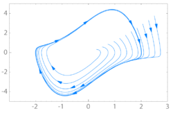
Stable limit cycle (shown in bold) and two other trajectories spiraling into it

Stable limit cycle (shown in bold) for the Van der Pol oscillator

In mathematics, in the study of dynamical systems with two-dimensional phase space, a limit cycle is a closed trajectory in phase space having the property that at least one other trajectory spirals into it either as time approaches infinity or as time approaches negative infinity. Such behavior is exhibited in some nonlinear systems. Limit cycles have been used to model the behavior of many real-world oscillatory systems. The study of limit cycles was initiated by Henri Poincaré (1854–1912).

Definition

We consider a two-dimensional dynamical system of the form

$${\displaystyle x'(t)=V(x(t))}$$

where

$${\displaystyle V:\mathbb {R} ^{2}\to \mathbb {R} ^{2}}$$

is a smooth function. A trajectory of this system is some smooth function ${\displaystyle x(t)}$ with values in ${\displaystyle \mathbb {R} ^{2}}$ which satisfies this differential equation. Such a trajectory is called closed (or periodic) if it is not constant but returns to its starting point, i.e. if there exists some ${\displaystyle t_{0}>0}$ such that ${\displaystyle x(t+t_{0})=x(t)}$ for all ${\displaystyle t\in \mathbb {R} }$. An orbit is the image of a trajectory, a subset of ${\displaystyle \mathbb {R} ^{2}}$. A closed orbit, or cycle, is the image of a closed trajectory. A limit cycle is a cycle which is the limit set of some other trajectory.

Properties

By the Jordan curve theorem, every closed trajectory divides the plane into two regions, the interior and the exterior of the curve.

Given a limit cycle and a trajectory in its interior that approaches the limit cycle for time approaching ${\displaystyle +\infty }$, then there is a neighborhood around the limit cycle such that all trajectories in the interior that start in the neighborhood approach the limit cycle for time approaching ${\displaystyle +\infty }$. The corresponding statement holds for a trajectory in the interior that approaches the limit cycle for time approaching ${\displaystyle -\infty }$, and also for trajectories in the exterior approaching the limit cycle.

Stable, unstable and semi-stable limit cycles

In the case where all the neighboring trajectories approach the limit cycle as time approaches infinity, it is called a stable or attractive limit cycle (ω-limit cycle). If instead, all neighboring trajectories approach it as time approaches negative infinity, then it is an unstable limit cycle (α-limit cycle). If there is a neighboring trajectory which spirals into the limit cycle as time approaches infinity, and another one which spirals into it as time approaches negative infinity, then it is a semi-stable limit cycle. There are also limit cycles that are neither stable, unstable nor semi-stable: for instance, a neighboring trajectory may approach the limit cycle from the outside, but the inside of the limit cycle is approached by a family of other cycles (which would not be limit cycles).

Stable limit cycles are examples of attractors. They imply self-sustained oscillations: the closed trajectory describes the perfect periodic behavior of the system, and any small perturbation from this closed trajectory causes the system to return to it, making the system stick to the limit cycle.

Finding limit cycles

Every closed trajectory contains within its interior a stationary point of the system, i.e. a point ${\displaystyle p}$ where ${\displaystyle V'(p)=0}$. The Bendixson–Dulac theorem and the Poincaré–Bendixson theorem predict the absence or existence, respectively, of limit cycles of two-dimensional nonlinear dynamical systems.

Open problems

Finding limit cycles, in general, is a very difficult problem. The number of limit cycles of a polynomial differential equation in the plane is the main object of the second part of Hilbert's sixteenth problem. It is unknown, for instance, whether there is any system ${\displaystyle x'=V(x)}$ in the plane where both components of ${\displaystyle V}$ are quadratic polynomials of the two variables, such that the system has more than 4 limit cycles.

Applications

Examples of limit cycles branching from fixed points near Hopf bifurcation. Trajectories in red, stable structures in dark blue, unstable structures in light blue. The parameter choice determines the occurrence and stability of limit cycles.

Limit cycles are important in many scientific applications where systems with self-sustained oscillations are modelled. Some examples include:

• Aerodynamic limit-cycle oscillations ^[1]
• The Hodgkin–Huxley model for action potentials in neurons.
• The Sel'kov model of glycolysis. ^[2]
• The daily oscillations in gene expression, hormone levels and body temperature of animals, which are part of the circadian rhythm, ^{[3] [4]} although this is contradicted by more recent evidence. ^[5]
• The migration of cancer cells in confining micro-environments follows limit cycle oscillations. ^[6]
• Some non-linear electrical circuits exhibit limit cycle oscillations, ^[7] which inspired the original Van der Pol model.
• The control of respiration and hematopoiesis, as appearing in the Mackey-Glass equations. ^[8]

See also

• Attractor
• Hyperbolic set
• Periodic point
• Self-oscillation
• Stable manifold

References

1. Thomas, Jeffrey P.; Dowell, Earl H.; Hall, Kenneth C. (2002), "Nonlinear Inviscid Aerodynamic Effects on Transonic Divergence, Flutter, and Limit-Cycle Oscillations" (PDF), AIAA Journal, 40 (4), American Institute of Aeronautics and Astronautics: 638, Bibcode:2002AIAAJ..40..638T, doi:10.2514/2.1720 , retrieved December 9, 2019
2. Sel'kov, E. E. (1968). "Self-Oscillations in Glycolysis 1. A Simple Kinetic Model". European Journal of Biochemistry. 4 (1): 79–86. doi: 10.1111/j.1432-1033.1968.tb00175.x . ISSN   1432-1033. PMID   4230812.
3. Leloup, Jean-Christophe; Gonze, Didier; Goldbeter, Albert (1999-12-01). "Limit Cycle Models for Circadian Rhythms Based on Transcriptional Regulation in Drosophila and Neurospora". Journal of Biological Rhythms. 14 (6): 433–448. doi:10.1177/074873099129000948. ISSN   0748-7304. PMID   10643740. S2CID   15074869.
4. Roenneberg, Till; Chua, Elaine Jane; Bernardo, Ric; Mendoza, Eduardo (2008-09-09). "Modelling Biological Rhythms". Current Biology. 18 (17): R826–R835. doi: 10.1016/j.cub.2008.07.017 . ISSN   0960-9822. PMID   18786388. S2CID   2798371.
5. Meijer, JH; Michel, S; Vanderleest, HT; Rohling, JH (December 2010). "Daily and seasonal adaptation of the circadian clock requires plasticity of the SCN neuronal network". The European Journal of Neuroscience. 32 (12): 2143–51. doi:10.1111/j.1460-9568.2010.07522.x. PMID   21143668. S2CID   12754517.
6. Brückner, David B.; Fink, Alexandra; Schreiber, Christoph; Röttgermann, Peter J. F.; Rädler, Joachim; Broedersz, Chase P. (2019). "Stochastic nonlinear dynamics of confined cell migration in two-state systems". Nature Physics. 15 (6): 595–601. Bibcode:2019NatPh..15..595B. doi:10.1038/s41567-019-0445-4. ISSN   1745-2481. S2CID   126819906.
7. Ginoux, Jean-Marc; Letellier, Christophe (2012-04-30). "Van der Pol and the history of relaxation oscillations: Toward the emergence of a concept". Chaos: An Interdisciplinary Journal of Nonlinear Science. 22 (2): 023120. arXiv: 1408.4890 . Bibcode:2012Chaos..22b3120G. doi:10.1063/1.3670008. ISSN   1054-1500. PMID   22757527. S2CID   293369.
8. Mackey, M.; Glass, L (1977-07-15). "Oscillation and chaos in physiological control systems". Science. 197 (4300): 287–289. Bibcode:1977Sci...197..287M. doi:10.1126/science.267326. ISSN   0036-8075. PMID   267326.

Further reading

• Steven H. Strogatz (2014). Nonlinear Dynamics and Chaos: With Applications to Physics, Biology, Chemistry, and Engineering. Avalon. ISBN   9780813349114.
• M. Vidyasagar (2002). Nonlinear Systems Analysis (Second ed.). SIAM. ISBN   9780898715262.
• Philip Hartman, "Ordinary Differential Equation", Society for Industrial and Applied Mathematics, 2002.
• Witold Hurewicz, "Lectures on Ordinary Differential Equations", Dover, 2002.
• Solomon Lefschetz, "Differential Equations: Geometric Theory", Dover, 2005.
• Lawrence Perko, "Differential Equations and Dynamical Systems", Springer-Verlag, 2006.
• Arthur Mattuck, Limit Cycles: Existence and Non-existence Criteria, MIT Open Courseware http://videolectures.net/mit1803s06_mattuck_lec32/#

External links

• "limit cycle". planetmath.org. Retrieved 2019-07-06.