Linear seismic inversion

Last updated

Inverse modeling is a mathematical technique where the objective is to determine the physical properties of the subsurface of an earth region that has produced a given seismogram. Cooke and Schneider (1983) [1] defined it as calculation of the earth’s structure and physical parameters from some set of observed seismic data. The underlying assumption in this method is that the collected seismic data are from an earth structure that matches the cross-section computed from the inversion algorithm. [2] Some common earth properties that are inverted for include acoustic velocity, formation and fluid densities, acoustic impedance, Poisson's ratio, formation compressibility, shear rigidity, porosity, and fluid saturation.

An inverse problem in science is the process of calculating from a set of observations the causal factors that produced them: for example, calculating an image in X-ray computed tomography, source reconstruction in acoustics, or calculating the density of the Earth from measurements of its gravity field.

Seismogram

A seismogram is a graph output by a seismograph. It is a record of the ground motion at a measuring station as a function of time. Seismograms typically record motions in three cartesian axes, with the z axis perpendicular to the Earth's surface and the x- and y- axes parallel to the surface. The energy measured in a seismogram may result from an earthquake or from some other source, such as an explosion. Seismograms can record lots of things, and record many little waves, called microseisms. These tiny microseisms can be caused by heavy traffic near the seismograph, waves hitting a beach, the wind, and any number of other ordinary things that cause some shaking of the seismograph.

Algorithm An unambiguous specification of how to solve a class of problems

In mathematics and computer science, an algorithm is an unambiguous specification of how to solve a class of problems. Algorithms can perform calculation, data processing, automated reasoning, and other tasks.

Contents

The method has long been useful for geophysicists and can be categorized into two broad types: [3] Deterministic and stochastic inversion. Deterministic inversion methods are based on comparison of the output from an earth model with the observed field data and continuously updating the earth model parameters to minimize a function, which is usually some form of difference between model output and field observation. As such, this method of inversion to which linear inversion falls under is posed as an minimization problem and the accepted earth model is the set of model parameters that minimizes the objective function in producing a numerical seismogram which best compares with collected field seismic data.

In computer science, a deterministic algorithm is an algorithm which, given a particular input, will always produce the same output, with the underlying machine always passing through the same sequence of states. Deterministic algorithms are by far the most studied and familiar kind of algorithm, as well as one of the most practical, since they can be run on real machines efficiently.

The word stochastic is an adjective in English that describes something that was randomly determined. The word first appeared in English to describe a mathematical object called a stochastic process, but now in mathematics the terms stochastic process and random process are considered interchangeable. The word, with its current definition meaning random, came from German, but it originally came from Greek στόχος (stókhos), meaning 'aim, guess'.

On the other hand, stochastic inversion methods are used to generate constrained models as used in reservoir flow simulation, using geostatistical tools like kriging. As opposed to deterministic inversion methods which produce a single set of model parameters, stochastic methods generate a suite of alternate earth model parameters which all obey the model constraint. However, the two methods are related as the results of deterministic models is the average of all the possible non-unique solutions of stochastic methods. [3] Since seismic linear inversion is a deterministic inversion method, the stochastic method will not be discussed beyond this point.

Reservoir A storage space for fluids

A reservoir is, most commonly, an enlarged natural or artificial lake, pond or impoundment created using a dam or lock to store water.

Kriging method of interpolation

In statistics, originally in geostatistics, kriging or Gaussian process regression is a method of interpolation for which the interpolated values are modeled by a Gaussian process governed by prior covariances. Under suitable assumptions on the priors, kriging gives the best linear unbiased prediction of the intermediate values. Interpolating methods based on other criteria such as smoothness need not yield the most likely intermediate values. The method is widely used in the domain of spatial analysis and computer experiments. The technique is also known as Wiener–Kolmogorov prediction, after Norbert Wiener and Andrey Kolmogorov.

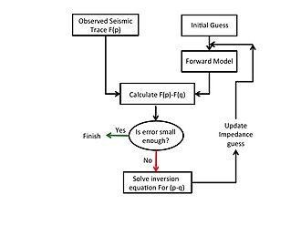
Figure 1: Linear Seismic Inversion Flow Chart Linear Seismic Inversion Flow Chart.jpg
Figure 1: Linear Seismic Inversion Flow Chart

Linear inversion

The deterministic nature of linear inversion requires a functional relationship which models, in terms of the earth model parameters, the seismic variable to be inverted. This functional relationship is some mathematical model derived from the fundamental laws of physics and is more often called a forward model. The aim of the technique is to minimize a function which is dependent on the difference between the convolution of the forward model with a source wavelet and the field collected seismic trace. As in the field of optimization, this function to be minimized is called the objective function and in convectional inverse modeling, is simply the difference between the convolved forward model and the seismic trace. As earlier mentioned, different types of variables can be inverted for but for clarity, these variables will be referred to as the impedance series of the earth model. In the following subsections we will describe in more detail, in the context of linear inversion as a minimization problem, the different components that are necessary to invert seismic data.

Function (mathematics) Mapping that associates a single output value to each input

In mathematics, a function was originally the idealization of how a varying quantity depends on another quantity. For example, the position of a planet is a function of time. Historically, the concept was elaborated with the infinitesimal calculus at the end of the 17th century, and, until the 19th century, the functions that were considered were differentiable. The concept of function was formalized at the end of the 19th century in terms of set theory, and this greatly enlarged the domains of application of the concept.

Wavelet function for integral Fourier-like transform

A wavelet is a wave-like oscillation with an amplitude that begins at zero, increases, and then decreases back to zero. It can typically be visualized as a "brief oscillation" like one recorded by a seismograph or heart monitor. Generally, wavelets are intentionally crafted to have specific properties that make them useful for signal processing. Using a "reverse, shift, multiply and integrate" technique called convolution, wavelets can be combined with known portions of a damaged signal to extract information from the unknown portions.

In seismology, a seismic trace refers to the recorded curve from a single seismograph when measuring ground movement. The name comes from the curve plotted by a seismograph as the paper roll rotated and the needle left a trace from which information about the subsurface could be extracted. Today's instruments record the data digitally and the word trace has come to mean the digital curve.

Forward model

The centerpiece of seismic linear inversion is the forward model which models the generation of the experimental data collected. [1] According to Wiggins (1972), [4] it provides a functional (computational) relationship between the model parameters and calculated values for the observed traces. Depending on the seismic data collected, this model may vary from the classical wave equations for predicting particle displacement or fluid pressure for sound wave propagation through rock or fluids, to some variants of these classical equations. For example, the forward model in Tarantola (1984) [5] is the wave equation for pressure variation in a liquid media during seismic wave propagation while by assuming constant velocity layers with plane interfaces, Kanasewich and Chiu (1985) [6] used the brachistotrone model of John Bernoulli for travel time of a ray along a path. In Cooke and Schneider (1983), [1] the model is a synthetic trace generation algorithm expressed as in Eqn. 3, where R(t) is generated in the Z-domain by recursive formula. In whatever form the forward model appears, it is important that it not only predicts the collected field data, but also models how the data is generated. Thus, the forward model by Cooke and Schneider (1983) [1] can only be used to invert CMP data since the model invariably assumes no spreading loss by mimicking the response of a laterally homogeneous earth to a plane-wave source

Wave equation Second-order linear differential equation important in physics

The wave equation is an important second-order linear partial differential equation for the description of waves—as they occur in classical physics—such as mechanical waves or light waves. It arises in fields like acoustics, electromagnetics, and fluid dynamics.

Particle displacement or displacement amplitude is a measurement of distance of the movement of a sound particle from its equilibrium position in a medium as it transmits a sound wave. The SI unit of particle displacement is the metre (m). In most cases this is a longitudinal wave of pressure, but it can also be a transverse wave, such as the vibration of a taut string. In the case of a sound wave travelling through air, the particle displacement is evident in the oscillations of air molecules with, and against, the direction in which the sound wave is travelling.

  1. where t is ray travel time, x, y, z are depth coordinates and vi is the constant velocity between interfaces i − 1 and i.
  2. where represent bulk modulus, density, the source of acoustic waves, and the pressure variation.

where s(t) = synthetic trace, w(t) = source wavelet, and R(t) = reflectivity function.

Objective function

An important numerical process in inverse modeling is to minimize the objective function, which is a function defined in terms of the difference between the collected field seismic data and the numerically computed seismic data. Classical objective functions include the sum of squared deviations between experimental and numerical data, as in the least squares methods, the sum of the magnitude of the difference between field and numerical data, or some variant of these definitions. Irrespective of the definition used, numerical solution of the inverse problem is obtained as earth model that minimize the objective function.

Least squares method in statistics

The method of least squares is a standard approach in regression analysis to approximate the solution of overdetermined systems, i.e., sets of equations in which there are more equations than unknowns. "Least squares" means that the overall solution minimizes the sum of the squares of the residuals made in the results of every single equation.

In mathematics, magnitude is the size of a mathematical object, a property which determines whether the object is larger or smaller than other objects of the same kind. More formally, an object's magnitude is the displayed result of an ordering of the class of objects to which it belongs.

In addition to the objective function, other constraints like known model parameters and known layer interfaces in some regions of the earth are also incorporated in the inverse modeling procedure. These constraints, according to Francis 2006, [3] help to reduce non-uniqueness of the inversion solution by providing a priori information that is not contained in the inverted data while Cooke and Schneider (1983) [1] reports their useful in controlling noise and when working in a geophysically well-known area.

Mathematical analysis of generalized linear inversion procedure

The objective of mathematical analysis of inverse modeling is to cast the generalized linear inverse problem into a simple matrix algebra by considering all the components described in previous sections. viz; forward model, objective function etc. Generally, the numerically generated seismic data are non-linear functions of the earth model parameters. To remove the non-linearity and create a platform for application of linear algebra concepts, the forward model is linearized by expansion using a Taylor series as carried out below. For more details see Wiggins (1972), [4] Cooke and Schneider (1983). [1]

Consider a set of seismic field observations , for and a set of earth model parameters to be inverted for, for . The field observations can be represented in either or , where and are vectorial representations of model parameters and the field observations as a function of earth parameters. Similarly, for representing guesses of model parameters, is the vector of numerical computed seismic data using the forward model of Sec. 1.3. Taylor's series expansion of about is given below.

  1. On linearization by dropping the non-linear terms (terms with (p⃗ − ⃗q) of order 2 and above), the equation becomes
  2. Considering that has components and and have components, the discrete form of Eqn. 5 results in a system of linear equations in variables whose matrix form is shown below.

is called the difference vector in Cooke and Schneider (1983). [1] It has a size of and its components are the difference between the observed trace and the numerically computed seismic data. is the corrector vector of size , while is called the sensitivity matrix. It has a size of and its comments are such that each column is the partial derivative of a component of the forward function with respect to one of the unknown earth model parameters. Similarly, each row is the partial derivative of a component of the numerically computed seismic trace with respect to all unknown model parameters.

Solution algorithm

is computed from the forward model, while is the experimental data. Thus, is a known quality. On the other hand, is unknown and is obtained by solution of Eqn. 10. This equation is theoretically solvable only when is invertible, that is, if it is a square matrix so that the number of observations is equal to the number of unknown earth parameters. If this is the case, the unknown corrector vector , is solved for as shown below, using any of the classical direct or iterative solvers for solution of a set of linear equations.

In most seismic inversion applications, there are more observations than the number of earth parameters to be inverted for, i.e. , leading to a system of equations that is mathematically over-determined. As a result, Eqn. 10 is not theoretically solvable and an exact solution is not obtainable. [6] An estimate of the corrector vector is obtained using the least squares procedure to find the corrector vector that minimizes , which is the sum of the squares of the error, . [6]

The error is given by

In the least squares procedure, the corrector vector that minimizes is obtained as below.

Thus,

From the above discussions, the objective function is defined as either the or norm of given by or or of given by or .

The generalized procedure for inverting any experimental seismic data for or , using the mathematical theory for inverse modeling, as described above, is shown in Fig. 1 and described as follows.

An initial guess of the model impedance is provided to initiate the inversion process. The forward model uses this initial guess to compute a synthetic seismic data which is subtracted from the observed seismic data to calculate the difference vector.

  1. An initial guess of the model impedance is provided to initiate the inversion process.
  2. A synthetic seismic data is computed by the forward model, using the model impedance above.
  3. The difference vector is computed as the difference between experimental and synthetic seismic data.
  4. The sensitivity matrix is computed at this value of the impedance profile.
  5. Using and the difference vector from 3 above, the corrector vector is calculated. A new impedance profile is obtained as
  6. The or norm of the computed corrector vector is compared with a provided tolerance value. If the computed norm is less than the tolerance, the numerical procedure is concluded and the inverted impedance profile for the earth region is given by from Eqn. 14. On the other hand, if the norm is greater than the tolerance, iterations through steps 2-6 are repeated but with an updated impedance profile as computed from Eqn. 14. Fig. 2 [7] shows a typical example of impedance profile updating during successive iteration process. According to Cooke and Schneider (1983), [1] use of the corrected guess from Eqn. 14 as the new initial guess during iteration reduces the error.

Parameterization of the earth model space

Irrespective of the variable to be inverted for, the earth’s impedance is a continuous function of depth (or time in seismic data) and for numerical linear inversion technique to be applicable for this continuous physical model, the continuous properties have to be discretized and/or sampled at discrete intervals along the depth of the earth model. Thus, the total depth over which model properties are to be determined is a necessary starting point for the discretization. Commonly, as shown in Fig. 3, this properties are sampled at close discrete intervals over this depth to ensure high resolution of impedance variation along the earth’s depth. The impedance values inverted from the algorithm represents the average value in the discrete interval.

Considering that inverse modeling problem is only theoretically solvable when the number of discrete intervals for sampling the properties is equal to the number of observation in the trace to be inverted, a high-resolution sampling will lead to a large matrix which will be very expensive to invert. Furthermore, the matrix may be singular for dependent equations, the inversion can be unstable in the presence of noise and the system may be under-constrained if parameters other than the primary variables inverted for, are desired. In relation to parameters desired, other than impedance, Cooke and Schneider (1983) [1] gives them to include source wavelet and scale factor.

Finally, by treating constraints as known impedance values in some layers or discrete intervals, the number of unknown impedance values to be solved for are reduced, leading to greater accuracy in the results of the inversion algorithm.

Figure 8:Amplitude Log Amplitude Log.jpg
Figure 8:Amplitude Log
Figure 9a:Impedance Logs Inverted From Amplitude Impedance Logs Inverted From Amplitude.jpg
Figure 9a:Impedance Logs Inverted From Amplitude
Figure 9b: Impedance Well Log Impedance Well Log.jpg
Figure 9b: Impedance Well Log

Inversion examples

Temperature inversion from Marescot (2010) [8]

We start with an example to invert for earth parameter values from temperature depth distribution in a given earth region. Although this example does not directly relate to seismic inversion since no traveling acoustic waves are involved, it nonetheless introduces practical application of the inversion technique in a manner easy to comprehend, before moving on to seismic applications. In this example, the temperature of the earth is measured at discrete locations in a well bore by placing temperature sensors in the target depths. By assuming a forward model of linear distribution of temperature with depth, two parameters are inverted for from the temperature depth measurements.

The forward model is given by

where . Thus, the dimension of is 2 i.e. the number of parameters inverted for is 2.

The objective of this inversion algorithm is to find , which is the value of that minimizes the difference between the observed temperature distribution and those obtained using the forward model of Eqn. 15. Considering the dimension of the forward model or the number of temperature observations to be , the components of the forward model is written as

  1. so that

We present results from Marescot (2010) [8] for the case of for which the observed temperature values at depths were at and at . These experimental data were inverted to obtain earth parameter values of and . For a more general case with large number of temperature observations, Fig. 4 shows the final linear forward model obtained from using the inverted values of and . The figure shows a good match between experimental and numerical data.

Wave travel time inversion from Marescot (2010) [8]

This examples inverts for earth layer velocity from recorded seismic wave travel times. Fig. 5 shows the initial velocity guesses and the travel times recorded from the field, while Fig. 6a shows the inverted heterogeneous velocity model, which is the solution of the inversion algorithm obtained after 30 iterations. As seen in Fig. 6b, there is good comparison between the final travel times obtained from the forward model using the inverted velocity and the field record travel times. Using these solutions, the ray path was reconstructed and is shown to be highly tortuous through the earth model as shown in Fig. 7.

Seismic trace inversion from Cooke and Schneider (1983)

This example, taken from Cooke and Schneider (1983), [1] shows inversion of a CMP seismic trace for earth model impedance (product of density and velocity) profile. The seismic trace inverted is shown in Fig. 8 while Fig. 9a shows the inverted impedance profile with the input initial impedance used for the inversion algorithm. Also recorded alongside the seismic trace is an impedance log of the earth region as shown in Fig. 9b. The figures show good comparison between the recorded impedance log and the numerical inverted impedance from the seismic trace.

Related Research Articles

Dirac delta function pseudo-function δ such that an integral of δ(x-c)f(x) always takes the value of f(c)

In mathematics, the Dirac delta function is a generalized function or distribution introduced by the physicist Paul Dirac. It is used to model the density of an idealized point mass or point charge as a function equal to zero everywhere except for zero and whose integral over the entire real line is equal to one. As there is no function that has these properties, the computations made by the theoretical physicists appeared to mathematicians as nonsense until the introduction of distributions by Laurent Schwartz to formalize and validate the computations. As a distribution, the Dirac delta function is a linear functional that maps every function to its value at zero. The Kronecker delta function, which is usually defined on a discrete domain and takes values 0 and 1, is a discrete analog of the Dirac delta function.

Noethers theorem Physical law that differentiable symmetries correspond to conservation laws

Noether's (first) theorem states that every differentiable symmetry of the action of a physical system has a corresponding conservation law. The theorem was proven by mathematician Emmy Noether in 1915 and published in 1918, after a special case was proven by E. Cosserat & F. Cosserat in 1909. The action of a physical system is the integral over time of a Lagrangian function, from which the system's behavior can be determined by the principle of least action. This theorem only applies to continuous and smooth symmetries over physical space.

Heat equation partial differential equation for distribution of heat in a given region over time

In physics and mathematics, the heat equation is a partial differential equation that describes how the distribution of some quantity evolves over time in a solid medium, as it spontaneously flows from places where it is higher towards places where it is lower. It is a special case of the diffusion equation.

Fokker–Planck equation Partial differential equation

In statistical mechanics, the Fokker–Planck equation is a partial differential equation that describes the time evolution of the probability density function of the velocity of a particle under the influence of drag forces and random forces, as in Brownian motion. The equation can be generalized to other observables as well. It is named after Adriaan Fokker and Max Planck, and is also known as the Kolmogorov forward equation, after Andrey Kolmogorov, who independently discovered the concept in 1931. When applied to particle position distributions, it is better known as the Smoluchowski equation, and in this context it is equivalent to the convection–diffusion equation. The case with zero diffusion is known in statistical mechanics as the Liouville equation. The Fokker–Planck equation is obtained from the master equation through Kramers–Moyal expansion.

Physical geodesy The study of the physical properties of the Earths gravity field

Physical geodesy is the study of the physical properties of the gravity field of the Earth, the geopotential, with a view to their application in geodesy.

In the mathematical field of differential geometry, a metric tensor is a type of function which takes as input a pair of tangent vectors v and w at a point of a surface and produces a real number scalar g(v, w) in a way that generalizes many of the familiar properties of the dot product of vectors in Euclidean space. In the same way as a dot product, metric tensors are used to define the length of and angle between tangent vectors. Through integration, the metric tensor allows one to define and compute the length of curves on the manifold.

Linear elasticity is the mathematical study of how solid objects deform and become internally stressed due to prescribed loading conditions. Linear elasticity models materials as continua. Linear elasticity is a simplification of the more general nonlinear theory of elasticity and is a branch of continuum mechanics. The fundamental "linearizing" assumptions of linear elasticity are: infinitesimal strains or "small" deformations and linear relationships between the components of stress and strain. In addition linear elasticity is valid only for stress states that do not produce yielding. These assumptions are reasonable for many engineering materials and engineering design scenarios. Linear elasticity is therefore used extensively in structural analysis and engineering design, often with the aid of finite element analysis.

In mathematics, the Hodge star operator or Hodge star is a linear map introduced by W. V. D. Hodge. It is defined on the exterior algebra of a finite-dimensional oriented vector space endowed with a nondegenerate symmetric bilinear form. The result when applied to an element of the algebra is called the element's Hodge dual.

In analytical mechanics, specifically the study of the rigid body dynamics of multibody systems, the term generalized coordinates refers to the parameters that describe the configuration of the system relative to some reference configuration. These parameters must uniquely define the configuration of the system relative to the reference configuration. This is done assuming that this can be done with a single chart. The generalized velocities are the time derivatives of the generalized coordinates of the system.

Rigid body dynamics studies the movement of systems of interconnected bodies under the action of external forces; described by the laws of kinematics and by the application of Newtons second law (kinetics) or their derivative form Lagrangian mechanics

Rigid-body dynamics studies the movement of systems of interconnected bodies under the action of external forces. The assumption that the bodies are rigid, which means that they do not deform under the action of applied forces, simplifies the analysis by reducing the parameters that describe the configuration of the system to the translation and rotation of reference frames attached to each body. This excludes bodies that display fluid, highly elastic, and plastic behavior.

Sound pressure or acoustic pressure is the local pressure deviation from the ambient atmospheric pressure, caused by a sound wave. In air, sound pressure can be measured using a microphone, and in water with a hydrophone. The SI unit of sound pressure is the pascal (Pa).

Acoustic impedance and specific acoustic impedance are measures of the opposition that a system presents to the acoustic flow resulting from an acoustic pressure applied to the system. The SI unit of acoustic impedance is the pascal second per cubic metre or the rayl per square metre, while that of specific acoustic impedance is the pascal second per metre or the rayl. In this article the symbol rayl denotes the MKS rayl. There is a close analogy with electrical impedance, which measures the opposition that a system presents to the electrical flow resulting from an electrical voltage applied to the system.

In mathematics, the Hamilton–Jacobi equation (HJE) is a necessary condition describing extremal geometry in generalizations of problems from the calculus of variations, and is a special case of the Hamilton–Jacobi–Bellman equation. It is named for William Rowan Hamilton and Carl Gustav Jacob Jacobi.

Total least squares

In applied statistics, total least squares is a type of errors-in-variables regression, a least squares data modeling technique in which observational errors on both dependent and independent variables are taken into account. It is a generalization of Deming regression and also of orthogonal regression, and can be applied to both linear and non-linear models.

Gauss–Newton algorithm algorithm

The Gauss–Newton algorithm is used to solve non-linear least squares problems. It is a modification of Newton's method for finding a minimum of a function. Unlike Newton's method, the Gauss–Newton algorithm can only be used to minimize a sum of squared function values, but it has the advantage that second derivatives, which can be challenging to compute, are not required.

Virtual work arises in the application of the principle of least action to the study of forces and movement of a mechanical system. The work of a force acting on a particle as it moves along a displacement is different for different displacements. Among all the possible displacements that a particle may follow, called virtual displacements, one will minimize the action. This displacement is therefore the displacement followed by the particle according to the principle of least action. The work of a force on a particle along a virtual displacement is known as the virtual work.

In differential geometry, the four-gradient is the four-vector analogue of the gradient from vector calculus.

In statistics, the generalized linear array model (GLAM) is used for analyzing data sets with array structures. It based on the generalized linear model with the design matrix written as a Kronecker product.

Non-linear least squares

Non-linear least squares is the form of least squares analysis used to fit a set of m observations with a model that is non-linear in n unknown parameters (m ≥ n). It is used in some forms of nonlinear regression. The basis of the method is to approximate the model by a linear one and to refine the parameters by successive iterations. There are many similarities to linear least squares, but also some significant differences. Examples of NLLS are (i) the Probit Regression, (ii) Threshold Regression, (iii) Smooth Regression, (iv) Logistic Link Regression, (v) Box-Cox Transformed Regressors, and many others in Economic Theory.

The transmission-line matrix (TLM) method is a space and time discretising method for computation of electromagnetic fields. It is based on the analogy between the electromagnetic field and a mesh of transmission lines. The TLM method allows the computation of complex three-dimensional electromagnetic structures and has proven to be one of the most powerful time-domain methods along with the finite difference time domain (FDTD) method.

References

  1. 1 2 3 4 5 6 7 8 9 10 Cooke, D. A.; Schneider W. A. (June 1983). "Generalized linear inversion of reflection seismic data". Geophysics. 48 (6): 665–676. doi:10.1190/1.1441497.
  2. Pica, A.; Diet J. P.; Tarantola A. (March 1990). "Nonlinear inversion of seismic reflection data in a laterally invariant medium". Geophysics. 55 (3): 284–292. doi:10.1190/1.1442836.
  3. 1 2 3 Francis, A.M. (November 2006). "Understanding Stochastic and Seismic Inversion". First Break. 24 (11). doi:10.3997/1365-2397.2006026.
  4. 1 2 Wiggins, Ralph (February 1972). "The general linear inverse problem: Implication of surface waves and free oscillations for Earth structure". Reviews of Geophysics. 10 (1): 251–285. doi:10.1029/RG010i001p00251.
  5. Tarantola, A. (1984). "Linearized and inversion of seismic reflection-data". Geophysical Prospecting. 32 (6): 908–1015. doi:10.1111/j.1365-2478.1984.tb00751.x.
  6. 1 2 3 Kanasewich, E. R.; Chiu S. K. L (June 1985). "Least squares inversion of spatial seismic refraction data". Bulletin of the Seismological Society of America. 75 (3): 865–880.
  7. Cooke, D; Cant J. (April 2010). "Model-based seismic inversion: Comparing deterministic and probabilistic approaches". CSEG Recorder.
  8. 1 2 3 Marescot, Laurent. "Introduction to Inversion in Geophysics" . Retrieved 3 May 2013.

Further reading