In linear algebra, the determinant is a scalar value that can be computed from the elements of a square matrix and encodes certain properties of the linear transformation described by the matrix. The determinant of a matrix A is denoted det(A), det A, or |A|. Geometrically, it can be viewed as the volume scaling factor of the linear transformation described by the matrix. This is also the signed volume of the n-dimensional parallelepiped spanned by the column or row vectors of the matrix. The determinant is positive or negative according to whether the linear mapping preserves or reverses the orientation of n-space.

In mathematical physics and mathematics, the Pauli matrices are a set of three 2 × 2 complex matrices which are Hermitian and unitary. Usually indicated by the Greek letter sigma, they are occasionally denoted by tau when used in connection with isospin symmetries. They are

Angular displacement of a body is the angle in radians through which a point revolves around a centre or line has been rotated in a specified sense about a specified axis. When a body rotates about its axis, the motion cannot simply be analyzed as a particle, as in circular motion it undergoes a changing velocity and acceleration at any time (t). When dealing with the rotation of a body, it becomes simpler to consider the body itself rigid. A body is generally considered rigid when the separations between all the particles remains constant throughout the body's motion, so for example parts of its mass are not flying off. In a realistic sense, all things can be deformable, however this impact is minimal and negligible. Thus the rotation of a rigid body over a fixed axis is referred to as rotational motion.

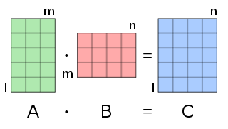
In mathematics, matrix multiplication is a binary operation that produces a matrix from two matrices. For matrix multiplication, the number of columns in the first matrix must be equal to the number of rows in the second matrix. The result matrix, known as the matrix product, has the number of rows of the first and the number of columns of the second matrix.
In linear algebra, the Cholesky decomposition or Cholesky factorization is a decomposition of a Hermitian, positive-definite matrix into the product of a lower triangular matrix and its conjugate transpose, which is useful for efficient numerical solutions, e.g., Monte Carlo simulations. It was discovered by André-Louis Cholesky for real matrices. When it is applicable, the Cholesky decomposition is roughly twice as efficient as the LU decomposition for solving systems of linear equations.

In linear algebra, the Cayley–Hamilton theorem states that every square matrix over a commutative ring satisfies its own characteristic equation.

In mathematics, the name symplectic group can refer to two different, but closely related, collections of mathematical groups, denoted Sp(2n, F) and Sp(n). The latter is called the compact symplectic group. Many authors prefer slightly different notations, usually differing by factors of 2. The notation used here is consistent with the size of the most common matrices which represent the groups. In Cartan's classification of the simple Lie algebras, the Lie algebra of the complex group Sp(2n, C) is denoted Cn, and Sp(n) is the compact real form of Sp(2n, C). Note that when we refer to the (compact) symplectic group it is implied that we are talking about the collection of (compact) symplectic groups, indexed by their dimension n.

In mathematics, the special unitary group of degree n, denoted SU(n), is the Lie group of n × n unitary matrices with determinant 1.

In special relativity, a four-vector is an object with four components, which transform in a specific way under Lorentz transformation. Specifically, a four-vector is an element of a four-dimensional vector space considered as a representation space of the standard representation of the Lorentz group, the (½,½) representation. It differs from a Euclidean vector in how its magnitude is determined. The transformations that preserve this magnitude are the Lorentz transformations, which include spatial rotations and boosts.
In linear algebra, a QR decomposition, also known as a QR factorization or QU factorization is a decomposition of a matrix A into a product A = QR of an orthogonal matrix Q and an upper triangular matrix R. QR decomposition is often used to solve the linear least squares problem and is the basis for a particular eigenvalue algorithm, the QR algorithm.
In mathematics, and in particular linear algebra, a pseudoinverse of a matrix is a generalization of the inverse matrix. The most widely known type of matrix pseudoinverse is the Moore–Penrose inverse, which was independently described by E. H. Moore in 1920, Arne Bjerhammar in 1951, and Roger Penrose in 1955. Earlier, Erik Ivar Fredholm had introduced the concept of a pseudoinverse of integral operators in 1903. When referring to a matrix, the term pseudoinverse, without further specification, is often used to indicate the Moore–Penrose inverse. The term generalized inverse is sometimes used as a synonym for pseudoinverse.
In mathematics, the Heisenberg group, named after Werner Heisenberg, is the group of 3×3 upper triangular matrices of the form

In classical cryptography, the Hill cipher is a polygraphic substitution cipher based on linear algebra. Invented by Lester S. Hill in 1929, it was the first polygraphic cipher in which it was practical to operate on more than three symbols at once. The following discussion assumes an elementary knowledge of matrices.
In linear algebra, a generalized eigenvector of an n × n matrix is a vector which satisfies certain criteria which are more relaxed than those for an (ordinary) eigenvector.
In mathematics, a hollow matrix may refer to one of several related classes of matrix.
In mathematics, the associative algebra of 2×2 real matrices is denoted by M(2, R). Two matrices p and q in M(2, R) have a sum p + q given by matrix addition. The product matrix p q is formed from the dot product of the rows and columns of its factors through matrix multiplication. For
In mathematics, specifically multilinear algebra, a dyadic or dyadic tensor is a second order tensor, written in a notation that fits in with vector algebra.
In the mathematical discipline of numerical linear algebra, a matrix splitting is an expression which represents a given matrix as a sum or difference of matrices. Many iterative methods depend upon the direct solution of matrix equations involving matrices more general than tridiagonal matrices. These matrix equations can often be solved directly and efficiently when written as a matrix splitting. The technique was devised by Richard S. Varga in 1960.
In numerical linear algebra, a convergent matrix is a matrix that converges to the zero matrix under matrix exponentiation.
In epidemiology, the next-generation matrix is a method used to derive the basic reproduction number, for a compartmental model of the spread of infectious diseases. This method is given by Diekmann et al. (1990) and van den Driessche and Watmough (2002). To calculate the basic reproduction number by using a next-generation matrix, the whole population is divided into compartments in which there are infected compartments. Let be the numbers of infected individuals in the infected compartment at time t. Now, the epidemic model is


