In statistics, the Gauss–Markov theorem states that the ordinary least squares (OLS) estimator has the lowest sampling variance within the class of linear unbiased estimators, if the errors in the linear regression model are uncorrelated, have equal variances and expectation value of zero. The errors do not need to be normal, nor do they need to be independent and identically distributed. The requirement that the estimator be unbiased cannot be dropped, since biased estimators exist with lower variance. See, for example, the James–Stein estimator, ridge regression, or simply any degenerate estimator.

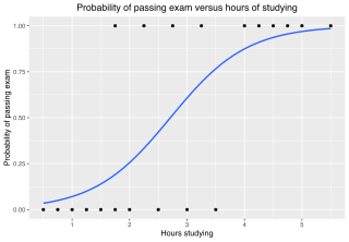
In statistics, the logistic model is a statistical model that models the log-odds of an event as a linear combination of one or more independent variables. In regression analysis, logistic regression estimates the parameters of a logistic model. In binary logistic regression there is a single binary dependent variable, coded by an indicator variable, where the two values are labeled "0" and "1", while the independent variables can each be a binary variable or a continuous variable. The corresponding probability of the value labeled "1" can vary between 0 and 1, hence the labeling; the function that converts log-odds to probability is the logistic function, hence the name. The unit of measurement for the log-odds scale is called a logit, from logistic unit, hence the alternative names. See § Background and § Definition for formal mathematics, and § Example for a worked example.
The Ising model, named after the physicists Ernst Ising and Wilhelm Lenz, is a mathematical model of ferromagnetism in statistical mechanics. The model consists of discrete variables that represent magnetic dipole moments of atomic "spins" that can be in one of two states. The spins are arranged in a graph, usually a lattice, allowing each spin to interact with its neighbors. Neighboring spins that agree have a lower energy than those that disagree; the system tends to the lowest energy but heat disturbs this tendency, thus creating the possibility of different structural phases. The model allows the identification of phase transitions as a simplified model of reality. The two-dimensional square-lattice Ising model is one of the simplest statistical models to show a phase transition.

In statistical modeling, regression analysis is a set of statistical processes for estimating the relationships between a dependent variable and one or more error-free independent variables.
In statistics, a linear probability model (LPM) is a special case of a binary regression model. Here the dependent variable for each observation takes values which are either 0 or 1. The probability of observing a 0 or 1 in any one case is treated as depending on one or more explanatory variables. For the "linear probability model", this relationship is a particularly simple one, and allows the model to be fitted by linear regression.
In statistics, a probit model is a type of regression where the dependent variable can take only two values, for example married or not married. The word is a portmanteau, coming from probability + unit. The purpose of the model is to estimate the probability that an observation with particular characteristics will fall into a specific one of the categories; moreover, classifying observations based on their predicted probabilities is a type of binary classification model.

In statistics, ordinary least squares (OLS) is a type of linear least squares method for choosing the unknown parameters in a linear regression model by the principle of least squares: minimizing the sum of the squares of the differences between the observed dependent variable in the input dataset and the output of the (linear) function of the independent variable. Some sources consider OLS to be linear regression.

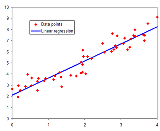
In statistics, simple linear regression (SLR) is a linear regression model with a single explanatory variable. That is, it concerns two-dimensional sample points with one independent variable and one dependent variable and finds a linear function that, as accurately as possible, predicts the dependent variable values as a function of the independent variable. The adjective simple refers to the fact that the outcome variable is related to a single predictor.
In statistics, multinomial logistic regression is a classification method that generalizes logistic regression to multiclass problems, i.e. with more than two possible discrete outcomes. That is, it is a model that is used to predict the probabilities of the different possible outcomes of a categorically distributed dependent variable, given a set of independent variables.
In statistics, generalized least squares (GLS) is a method used to estimate the unknown parameters in a linear regression model. It is used when there is a non-zero amount of correlation between the residuals in the regression model. GLS is employed to improve statistical efficiency and reduce the risk of drawing erroneous inferences, as compared to conventional least squares and weighted least squares methods. It was first described by Alexander Aitken in 1935.
In economics, discrete choice models, or qualitative choice models, describe, explain, and predict choices between two or more discrete alternatives, such as entering or not entering the labor market, or choosing between modes of transport. Such choices contrast with standard consumption models in which the quantity of each good consumed is assumed to be a continuous variable. In the continuous case, calculus methods can be used to determine the optimum amount chosen, and demand can be modeled empirically using regression analysis. On the other hand, discrete choice analysis examines situations in which the potential outcomes are discrete, such that the optimum is not characterized by standard first-order conditions. Thus, instead of examining "how much" as in problems with continuous choice variables, discrete choice analysis examines "which one". However, discrete choice analysis can also be used to examine the chosen quantity when only a few distinct quantities must be chosen from, such as the number of vehicles a household chooses to own and the number of minutes of telecommunications service a customer decides to purchase. Techniques such as logistic regression and probit regression can be used for empirical analysis of discrete choice.
In statistics, binomial regression is a regression analysis technique in which the response has a binomial distribution: it is the number of successes in a series of independent Bernoulli trials, where each trial has probability of success . In binomial regression, the probability of a success is related to explanatory variables: the corresponding concept in ordinary regression is to relate the mean value of the unobserved response to explanatory variables.
In statistics and econometrics, the multivariate probit model is a generalization of the probit model used to estimate several correlated binary outcomes jointly. For example, if it is believed that the decisions of sending at least one child to public school and that of voting in favor of a school budget are correlated, then the multivariate probit model would be appropriate for jointly predicting these two choices on an individual-specific basis. J.R. Ashford and R.R. Sowden initially proposed an approach for multivariate probit analysis. Siddhartha Chib and Edward Greenberg extended this idea and also proposed simulation-based inference methods for the multivariate probit model which simplified and generalized parameter estimation.
The topic of heteroskedasticity-consistent (HC) standard errors arises in statistics and econometrics in the context of linear regression and time series analysis. These are also known as heteroskedasticity-robust standard errors, Eicker–Huber–White standard errors, to recognize the contributions of Friedhelm Eicker, Peter J. Huber, and Halbert White.
In statistics and econometrics, the multinomial probit model is a generalization of the probit model used when there are several possible categories that the dependent variable can fall into. As such, it is an alternative to the multinomial logit model as one method of multiclass classification. It is not to be confused with the multivariate probit model, which is used to model correlated binary outcomes for more than one independent variable.
Although the concept choice models is widely understood and practiced these days, it is often difficult to acquire hands-on knowledge in simulating choice models. While many stat packages provide useful tools to simulate, researchers attempting to test and simulate new choice models with data often encounter problems from as simple as scaling parameter to misspecification. This article goes beyond simply defining discrete choice models. Rather, it aims at providing a comprehensive overview of how to simulate such models in computer.

In statistics, polynomial regression is a form of regression analysis in which the relationship between the independent variable x and the dependent variable y is modeled as an nth degree polynomial in x. Polynomial regression fits a nonlinear relationship between the value of x and the corresponding conditional mean of y, denoted E(y |x). Although polynomial regression fits a nonlinear model to the data, as a statistical estimation problem it is linear, in the sense that the regression function E(y | x) is linear in the unknown parameters that are estimated from the data. For this reason, polynomial regression is considered to be a special case of multiple linear regression.
In statistics and econometrics, the maximum score estimator is a nonparametric estimator for discrete choice models developed by Charles Manski in 1975. Unlike the multinomial probit and multinomial logit estimators, it makes no assumptions about the distribution of the unobservable part of utility. However, its statistical properties are more complicated than the multinomial probit and logit models, making statistical inference difficult. To address these issues, Joel Horowitz proposed a variant, called the smoothed maximum score estimator.
In statistics, linear regression is a model that estimates the linear relationship between a scalar response and one or more explanatory variables. A model with exactly one explanatory variable is a simple linear regression; a model with two or more explanatory variables is a multiple linear regression. This term is distinct from multivariate linear regression, which predicts multiple correlated dependent variables rather than a single dependent variable.
Dynamic discrete choice (DDC) models, also known as discrete choice models of dynamic programming, model an agent's choices over discrete options that have future implications. Rather than assuming observed choices are the result of static utility maximization, observed choices in DDC models are assumed to result from an agent's maximization of the present value of utility, generalizing the utility theory upon which discrete choice models are based.


