Related Research Articles
In mathematics, a dynamical system is a system in which a function describes the time dependence of a point in an ambient space, such as in a parametric curve. Examples include the mathematical models that describe the swinging of a clock pendulum, the flow of water in a pipe, the random motion of particles in the air, and the number of fish each springtime in a lake. The most general definition unifies several concepts in mathematics such as ordinary differential equations and ergodic theory by allowing different choices of the space and how time is measured. Time can be measured by integers, by real or complex numbers or can be a more general algebraic object, losing the memory of its physical origin, and the space may be a manifold or simply a set, without the need of a smooth space-time structure defined on it.

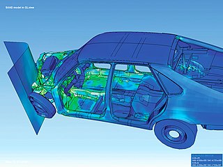
Computational fluid dynamics (CFD) is a branch of fluid mechanics that uses numerical analysis and data structures to analyze and solve problems that involve fluid flows. Computers are used to perform the calculations required to simulate the free-stream flow of the fluid, and the interaction of the fluid with surfaces defined by boundary conditions. With high-speed supercomputers, better solutions can be achieved, and are often required to solve the largest and most complex problems. Ongoing research yields software that improves the accuracy and speed of complex simulation scenarios such as transonic or turbulent flows. Initial validation of such software is typically performed using experimental apparatus such as wind tunnels. In addition, previously performed analytical or empirical analysis of a particular problem can be used for comparison. A final validation is often performed using full-scale testing, such as flight tests.
In plasma physics, the particle-in-cell (PIC) method refers to a technique used to solve a certain class of partial differential equations. In this method, individual particles in a Lagrangian frame are tracked in continuous phase space, whereas moments of the distribution such as densities and currents are computed simultaneously on Eulerian (stationary) mesh points.
Numerical methods for partial differential equations is the branch of numerical analysis that studies the numerical solution of partial differential equations (PDEs).
In numerical analysis, adaptive mesh refinement (AMR) is a method of adapting the accuracy of a solution within certain sensitive or turbulent regions of simulation, dynamically and during the time the solution is being calculated. When solutions are calculated numerically, they are often limited to pre-determined quantified grids as in the Cartesian plane which constitute the computational grid, or 'mesh'. Many problems in numerical analysis, however, do not require a uniform precision in the numerical grids used for graph plotting or computational simulation, and would be better suited if specific areas of graphs which needed precision could be refined in quantification only in the regions requiring the added precision. Adaptive mesh refinement provides such a dynamic programming environment for adapting the precision of the numerical computation based on the requirements of a computation problem in specific areas of multi-dimensional graphs which need precision while leaving the other regions of the multi-dimensional graphs at lower levels of precision and resolution.

Finite-difference time-domain (FDTD) or Yee's method is a numerical analysis technique used for modeling computational electrodynamics. Since it is a time-domain method, FDTD solutions can cover a wide frequency range with a single simulation run, and treat nonlinear material properties in a natural way.

Mesh generation is the practice of creating a mesh, a subdivision of a continuous geometric space into discrete geometric and topological cells. Often these cells form a simplicial complex. Usually the cells partition the geometric input domain. Mesh cells are used as discrete local approximations of the larger domain. Meshes are created by computer algorithms, often with human guidance through a GUI, depending on the complexity of the domain and the type of mesh desired. A typical goal is to create a mesh that accurately captures the input domain geometry, with high-quality (well-shaped) cells, and without so many cells as to make subsequent calculations intractable. The mesh should also be fine in areas that are important for the subsequent calculations.

Computational electromagnetics (CEM), computational electrodynamics or electromagnetic modeling is the process of modeling the interaction of electromagnetic fields with physical objects and the environment.

Soft-body dynamics is a field of computer graphics that focuses on visually realistic physical simulations of the motion and properties of deformable objects. The applications are mostly in video games and films. Unlike in simulation of rigid bodies, the shape of soft bodies can change, meaning that the relative distance of two points on the object is not fixed. While the relative distances of points are not fixed, the body is expected to retain its shape to some degree. The scope of soft body dynamics is quite broad, including simulation of soft organic materials such as muscle, fat, hair and vegetation, as well as other deformable materials such as clothing and fabric. Generally, these methods only provide visually plausible emulations rather than accurate scientific/engineering simulations, though there is some crossover with scientific methods, particularly in the case of finite element simulations. Several physics engines currently provide software for soft-body simulation.

In numerical analysis, finite-difference methods (FDM) are a class of numerical techniques for solving differential equations by approximating derivatives with finite differences. Both the spatial domain and time interval are discretized, or broken into a finite number of steps, and the value of the solution at these discrete points is approximated by solving algebraic equations containing finite differences and values from nearby points.

In the field of numerical analysis, meshfree methods are those that do not require connection between nodes of the simulation domain, i.e. a mesh, but are rather based on interaction of each node with all its neighbors. As a consequence, original extensive properties such as mass or kinetic energy are no longer assigned to mesh elements but rather to the single nodes. Meshfree methods enable the simulation of some otherwise difficult types of problems, at the cost of extra computing time and programming effort. The absence of a mesh allows Lagrangian simulations, in which the nodes can move according to the velocity field.
The finite-difference frequency-domain (FDFD) method is a numerical solution method for problems usually in electromagnetism and sometimes in acoustics, based on finite-difference approximations of the derivative operators in the differential equation being solved.
The material point method (MPM) is a numerical technique used to simulate the behavior of solids, liquids, gases, and any other continuum material. Especially, it is a robust spatial discretization method for simulating multi-phase (solid-fluid-gas) interactions. In the MPM, a continuum body is described by a number of small Lagrangian elements referred to as 'material points'. These material points are surrounded by a background mesh/grid that is used to calculate terms such as the deformation gradient. Unlike other mesh-based methods like the finite element method, finite volume method or finite difference method, the MPM is not a mesh based method and is instead categorized as a meshless/meshfree or continuum-based particle method, examples of which are smoothed particle hydrodynamics and peridynamics. Despite the presence of a background mesh, the MPM does not encounter the drawbacks of mesh-based methods which makes it a promising and powerful tool in computational mechanics.
The finite element method (FEM) is a popular method for numerically solving differential equations arising in engineering and mathematical modeling. Typical problem areas of interest include the traditional fields of structural analysis, heat transfer, fluid flow, mass transport, and electromagnetic potential.
False diffusion is a type of error observed when the upwind scheme is used to approximate the convection term in convection–diffusion equations. The more accurate central difference scheme can be used for the convection term, but for grids with cell Peclet number more than 2, the central difference scheme is unstable and the simpler upwind scheme is often used. The resulting error from the upwind differencing scheme has a diffusion-like appearance in two- or three-dimensional co-ordinate systems and is referred as "false diffusion". False-diffusion errors in numerical solutions of convection-diffusion problems, in two- and three-dimensions, arise from the numerical approximations of the convection term in the conservation equations. Over the past 20 years many numerical techniques have been developed to solve convection-diffusion equations and none are problem-free, but false diffusion is one of the most serious problems and a major topic of controversy and confusion among numerical analysts.
Equation-free modeling is a method for multiscale computation and computer-aided analysis. It is designed for a class of complicated systems in which one observes evolution at a macroscopic, coarse scale of interest, while accurate models are only given at a finely detailed, microscopic, level of description. The framework empowers one to perform macroscopic computational tasks using only appropriately initialized microscopic simulation on short time and small length scales. The methodology eliminates the derivation of explicit macroscopic evolution equations when these equations conceptually exist but are not available in closed form; hence the term equation-free.
Fluid motion is governed by the Navier–Stokes equations, a set of coupled and nonlinear partial differential equations derived from the basic laws of conservation of mass, momentum and energy. The unknowns are usually the flow velocity, the pressure and density and temperature. The analytical solution of this equation is impossible hence scientists resort to laboratory experiments in such situations. The answers delivered are, however, usually qualitatively different since dynamical and geometric similitude are difficult to enforce simultaneously between the lab experiment and the prototype. Furthermore, the design and construction of these experiments can be difficult, particularly for stratified rotating flows. Computational fluid dynamics (CFD) is an additional tool in the arsenal of scientists. In its early days CFD was often controversial, as it involved additional approximation to the governing equations and raised additional (legitimate) issues. Nowadays CFD is an established discipline alongside theoretical and experimental methods. This position is in large part due to the exponential growth of computer power which has allowed us to tackle ever larger and more complex problems.
Ocean general circulation models (OGCMs) are a particular kind of general circulation model to describe physical and thermodynamical processes in oceans. The oceanic general circulation is defined as the horizontal space scale and time scale larger than mesoscale. They depict oceans using a three-dimensional grid that include active thermodynamics and hence are most directly applicable to climate studies. They are the most advanced tools currently available for simulating the response of the global ocean system to increasing greenhouse gas concentrations. A hierarchy of OGCMs have been developed that include varying degrees of spatial coverage, resolution, geographical realism, process detail, etc.

In geology, numerical modeling is a widely applied technique to tackle complex geological problems by computational simulation of geological scenarios.
References
- ↑ Hyman, J.M. (2005). "Patch dynamics for multiscale problems". Computing in Science & Engineering. 7 (3): 47–53. Bibcode:2005CSE.....7c..47H. CiteSeerX 10.1.1.454.6285 . doi:10.1109/MCSE.2005.57. S2CID 2654914.
| | This fluid dynamics–related article is a stub. You can help Wikipedia by expanding it. |