
In mathematical physics and mathematics, the Pauli matrices are a set of three 2 × 2 complex matrices that are Hermitian, involutory and unitary. Usually indicated by the Greek letter sigma, they are occasionally denoted by tau when used in connection with isospin symmetries.

In statistical mechanics and information theory, the Fokker–Planck equation is a partial differential equation that describes the time evolution of the probability density function of the velocity of a particle under the influence of drag forces and random forces, as in Brownian motion. The equation can be generalized to other observables as well. The Fokker-Planck equation has multiple applications in information theory, graph theory, data science, finance, economics etc.
Linear elasticity is a mathematical model of how solid objects deform and become internally stressed due to prescribed loading conditions. It is a simplification of the more general nonlinear theory of elasticity and a branch of continuum mechanics.
A Newtonian fluid is a fluid in which the viscous stresses arising from its flow are at every point linearly correlated to the local strain rate — the rate of change of its deformation over time. Stresses are proportional to the rate of change of the fluid's velocity vector.
A directional derivative is a concept in multivariable calculus that measures the rate at which a function changes in a particular direction at a given point.

In quantum mechanics and quantum field theory, the propagator is a function that specifies the probability amplitude for a particle to travel from one place to another in a given period of time, or to travel with a certain energy and momentum. In Feynman diagrams, which serve to calculate the rate of collisions in quantum field theory, virtual particles contribute their propagator to the rate of the scattering event described by the respective diagram. Propagators may also be viewed as the inverse of the wave operator appropriate to the particle, and are, therefore, often called (causal) Green's functions.
In physics, the Hamilton–Jacobi equation, named after William Rowan Hamilton and Carl Gustav Jacob Jacobi, is an alternative formulation of classical mechanics, equivalent to other formulations such as Newton's laws of motion, Lagrangian mechanics and Hamiltonian mechanics.

In nuclear physics, the chiral model, introduced by Feza Gürsey in 1960, is a phenomenological model describing effective interactions of mesons in the chiral limit (where the masses of the quarks go to zero), but without necessarily mentioning quarks at all. It is a nonlinear sigma model with the principal homogeneous space of a Lie group as its target manifold. When the model was originally introduced, this Lie group was the SU(N), where N is the number of quark flavors. The Riemannian metric of the target manifold is given by a positive constant multiplied by the Killing form acting upon the Maurer–Cartan form of SU(N).
In statistics, econometrics, and signal processing, an autoregressive (AR) model is a representation of a type of random process; as such, it is used to describe certain time-varying processes in nature, economics, behavior, etc. The autoregressive model specifies that the output variable depends linearly on its own previous values and on a stochastic term ; thus the model is in the form of a stochastic difference equation which should not be confused with a differential equation. Together with the moving-average (MA) model, it is a special case and key component of the more general autoregressive–moving-average (ARMA) and autoregressive integrated moving average (ARIMA) models of time series, which have a more complicated stochastic structure; it is also a special case of the vector autoregressive model (VAR), which consists of a system of more than one interlocking stochastic difference equation in more than one evolving random variable.
In linear algebra, the Laplace expansion, named after Pierre-Simon Laplace, also called cofactor expansion, is an expression of the determinant of an n × n-matrix B as a weighted sum of minors, which are the determinants of some (n − 1) × (n − 1)-submatrices of B. Specifically, for every i, the Laplace expansion along the ith row is the equality
In theoretical physics, Seiberg–Witten theory is an supersymmetric gauge theory with an exact low-energy effective action, of which the kinetic part coincides with the Kähler potential of the moduli space of vacua. Before taking the low-energy effective action, the theory is known as supersymmetric Yang–Mills theory, as the field content is a single vector supermultiplet, analogous to the field content of Yang–Mills theory being a single vector gauge field or connection.

In complex analysis, a branch of mathematics, a holomorphic function is said to be of exponential type C if its growth is bounded by the exponential function for some real-valued constant as . When a function is bounded in this way, it is then possible to express it as certain kinds of convergent summations over a series of other complex functions, as well as understanding when it is possible to apply techniques such as Borel summation, or, for example, to apply the Mellin transform, or to perform approximations using the Euler–Maclaurin formula. The general case is handled by Nachbin's theorem, which defines the analogous notion of -type for a general function as opposed to .
The Newman–Penrose (NP) formalism is a set of notation developed by Ezra T. Newman and Roger Penrose for general relativity (GR). Their notation is an effort to treat general relativity in terms of spinor notation, which introduces complex forms of the usual variables used in GR. The NP formalism is itself a special case of the tetrad formalism, where the tensors of the theory are projected onto a complete vector basis at each point in spacetime. Usually this vector basis is chosen to reflect some symmetry of the spacetime, leading to simplified expressions for physical observables. In the case of the NP formalism, the vector basis chosen is a null tetrad: a set of four null vectors—two real, and a complex-conjugate pair. The two real members often asymptotically point radially inward and radially outward, and the formalism is well adapted to treatment of the propagation of radiation in curved spacetime. The Weyl scalars, derived from the Weyl tensor, are often used. In particular, it can be shown that one of these scalars— in the appropriate frame—encodes the outgoing gravitational radiation of an asymptotically flat system.
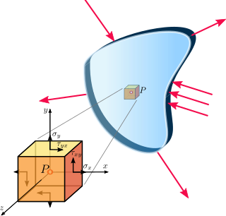
In continuum mechanics, a material is said to be under plane stress if the stress vector is zero across a particular plane. When that situation occurs over an entire element of a structure, as is often the case for thin plates, the stress analysis is considerably simplified, as the stress state can be represented by a tensor of dimension 2. A related notion, plane strain, is often applicable to very thick members.

Viscoplasticity is a theory in continuum mechanics that describes the rate-dependent inelastic behavior of solids. Rate-dependence in this context means that the deformation of the material depends on the rate at which loads are applied. The inelastic behavior that is the subject of viscoplasticity is plastic deformation which means that the material undergoes unrecoverable deformations when a load level is reached. Rate-dependent plasticity is important for transient plasticity calculations. The main difference between rate-independent plastic and viscoplastic material models is that the latter exhibit not only permanent deformations after the application of loads but continue to undergo a creep flow as a function of time under the influence of the applied load.
In mathematics, the oscillator representation is a projective unitary representation of the symplectic group, first investigated by Irving Segal, David Shale, and André Weil. A natural extension of the representation leads to a semigroup of contraction operators, introduced as the oscillator semigroup by Roger Howe in 1988. The semigroup had previously been studied by other mathematicians and physicists, most notably Felix Berezin in the 1960s. The simplest example in one dimension is given by SU(1,1). It acts as Möbius transformations on the extended complex plane, leaving the unit circle invariant. In that case the oscillator representation is a unitary representation of a double cover of SU(1,1) and the oscillator semigroup corresponds to a representation by contraction operators of the semigroup in SL(2,C) corresponding to Möbius transformations that take the unit disk into itself.
In quantum field theory, and in the significant subfields of quantum electrodynamics (QED) and quantum chromodynamics (QCD), the two-body Dirac equations (TBDE) of constraint dynamics provide a three-dimensional yet manifestly covariant reformulation of the Bethe–Salpeter equation for two spin-1/2 particles. Such a reformulation is necessary since without it, as shown by Nakanishi, the Bethe–Salpeter equation possesses negative-norm solutions arising from the presence of an essentially relativistic degree of freedom, the relative time. These "ghost" states have spoiled the naive interpretation of the Bethe–Salpeter equation as a quantum mechanical wave equation. The two-body Dirac equations of constraint dynamics rectify this flaw. The forms of these equations can not only be derived from quantum field theory they can also be derived purely in the context of Dirac's constraint dynamics and relativistic mechanics and quantum mechanics. Their structures, unlike the more familiar two-body Dirac equation of Breit, which is a single equation, are that of two simultaneous quantum relativistic wave equations. A single two-body Dirac equation similar to the Breit equation can be derived from the TBDE. Unlike the Breit equation, it is manifestly covariant and free from the types of singularities that prevent a strictly nonperturbative treatment of the Breit equation. In applications of the TBDE to QED, the two particles interact by way of four-vector potentials derived from the field theoretic electromagnetic interactions between the two particles. In applications to QCD, the two particles interact by way of four-vector potentials and Lorentz invariant scalar interactions, derived in part from the field theoretic chromomagnetic interactions between the quarks and in part by phenomenological considerations. As with the Breit equation a sixteen-component spinor Ψ is used.
In mathematics, the Fuglede−Kadison determinant of an invertible operator in a finite factor is a positive real number associated with it. It defines a multiplicative homomorphism from the set of invertible operators to the set of positive real numbers. The Fuglede−Kadison determinant of an operator is often denoted by .
In mathematics, the injective tensor product of two topological vector spaces (TVSs) was introduced by Alexander Grothendieck and was used by him to define nuclear spaces. An injective tensor product is in general not necessarily complete, so its completion is called the completed injective tensor products. Injective tensor products have applications outside of nuclear spaces. In particular, as described below, up to TVS-isomorphism, many TVSs that are defined for real or complex valued functions, for instance, the Schwartz space or the space of continuously differentiable functions, can be immediately extended to functions valued in a Hausdorff locally convex TVS without any need to extend definitions from real/complex-valued functions to -valued functions.

In mathematics, the Chambolle-Pock algorithm is an algorithm used to solve convex optimization problems. It was introduced by Antonin Chambolle and Thomas Pock in 2011 and has since become a widely used method in various fields, including image processing, computer vision, and signal processing.


