
The method of least squares is a standard approach in regression analysis to approximate the solution of overdetermined systems by minimizing the sum of the squares of the residuals made in the results of each individual equation.
In mathematical modeling, overfitting is "the production of an analysis that corresponds too closely or exactly to a particular set of data, and may therefore fail to fit to additional data or predict future observations reliably". An overfitted model is a mathematical model that contains more parameters than can be justified by the data. The essence of overfitting is to have unknowingly extracted some of the residual variation as if that variation represented underlying model structure.

In statistics, the logistic model is a statistical model that models the probability of an event taking place by having the log-odds for the event be a linear combination of one or more independent variables. In regression analysis, logistic regression is estimating the parameters of a logistic model. Formally, in binary logistic regression there is a single binary dependent variable, coded by an indicator variable, where the two values are labeled "0" and "1", while the independent variables can each be a binary variable or a continuous variable. The corresponding probability of the value labeled "1" can vary between 0 and 1, hence the labeling; the function that converts log-odds to probability is the logistic function, hence the name. The unit of measurement for the log-odds scale is called a logit, from logistic unit, hence the alternative names. See § Background and § Definition for formal mathematics, and § Example for a worked example.

In mathematics, a time series is a series of data points indexed in time order. Most commonly, a time series is a sequence taken at successive equally spaced points in time. Thus it is a sequence of discrete-time data. Examples of time series are heights of ocean tides, counts of sunspots, and the daily closing value of the Dow Jones Industrial Average.
In statistics, deviance is a goodness-of-fit statistic for a statistical model; it is often used for statistical hypothesis testing. It is a generalization of the idea of using the sum of squares of residuals (SSR) in ordinary least squares to cases where model-fitting is achieved by maximum likelihood. It plays an important role in exponential dispersion models and generalized linear models.

Curve fitting is the process of constructing a curve, or mathematical function, that has the best fit to a series of data points, possibly subject to constraints. Curve fitting can involve either interpolation, where an exact fit to the data is required, or smoothing, in which a "smooth" function is constructed that approximately fits the data. A related topic is regression analysis, which focuses more on questions of statistical inference such as how much uncertainty is present in a curve that is fit to data observed with random errors. Fitted curves can be used as an aid for data visualization, to infer values of a function where no data are available, and to summarize the relationships among two or more variables. Extrapolation refers to the use of a fitted curve beyond the range of the observed data, and is subject to a degree of uncertainty since it may reflect the method used to construct the curve as much as it reflects the observed data.

In statistics, nonlinear regression is a form of regression analysis in which observational data are modeled by a function which is a nonlinear combination of the model parameters and depends on one or more independent variables. The data are fitted by a method of successive approximations.
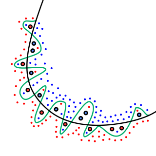
Random sample consensus (RANSAC) is an iterative method to estimate parameters of a mathematical model from a set of observed data that contains outliers, when outliers are to be accorded no influence on the values of the estimates. Therefore, it also can be interpreted as an outlier detection method. It is a non-deterministic algorithm in the sense that it produces a reasonable result only with a certain probability, with this probability increasing as more iterations are allowed. The algorithm was first published by Fischler and Bolles at SRI International in 1981. They used RANSAC to solve the Location Determination Problem (LDP), where the goal is to determine the points in the space that project onto an image into a set of landmarks with known locations.
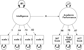
Structural equation modeling (SEM) is a label for a diverse set of methods used by scientists in both experimental and observational research across the sciences, business, and other fields. It is used most in the social and behavioral sciences. A definition of SEM is difficult without reference to highly technical language, but a good starting place is the name itself.
In statistics, a generalized additive model (GAM) is a generalized linear model in which the linear response variable depends linearly on unknown smooth functions of some predictor variables, and interest focuses on inference about these smooth functions.

Local regression or local polynomial regression, also known as moving regression, is a generalization of the moving average and polynomial regression. Its most common methods, initially developed for scatterplot smoothing, are LOESS and LOWESS, both pronounced. They are two strongly related non-parametric regression methods that combine multiple regression models in a k-nearest-neighbor-based meta-model. In some fields, LOESS is known and commonly referred to as Savitzky–Golay filter.
Omnibus tests are a kind of statistical test. They test whether the explained variance in a set of data is significantly greater than the unexplained variance, overall. One example is the F-test in the analysis of variance. There can be legitimate significant effects within a model even if the omnibus test is not significant. For instance, in a model with two independent variables, if only one variable exerts a significant effect on the dependent variable and the other does not, then the omnibus test may be non-significant. This fact does not affect the conclusions that may be drawn from the one significant variable. In order to test effects within an omnibus test, researchers often use contrasts.
In statistics, the restrictedmaximum likelihood (REML) approach is a particular form of maximum likelihood estimation that does not base estimates on a maximum likelihood fit of all the information, but instead uses a likelihood function calculated from a transformed set of data, so that nuisance parameters have no effect.
In statistics, a generalized linear mixed model (GLMM) is an extension to the generalized linear model (GLM) in which the linear predictor contains random effects in addition to the usual fixed effects. They also inherit from GLMs the idea of extending linear mixed models to non-normal data.
In statistics, identifiability is a property which a model must satisfy for precise inference to be possible. A model is identifiable if it is theoretically possible to learn the true values of this model's underlying parameters after obtaining an infinite number of observations from it. Mathematically, this is equivalent to saying that different values of the parameters must generate different probability distributions of the observable variables. Usually the model is identifiable only under certain technical restrictions, in which case the set of these requirements is called the identification conditions.
Linear least squares (LLS) is the least squares approximation of linear functions to data. It is a set of formulations for solving statistical problems involved in linear regression, including variants for ordinary (unweighted), weighted, and generalized (correlated) residuals. Numerical methods for linear least squares include inverting the matrix of the normal equations and orthogonal decomposition methods.
In statistics Wilks' theorem offers an asymptotic distribution of the log-likelihood ratio statistic, which can be used to produce confidence intervals for maximum-likelihood estimates or as a test statistic for performing the likelihood-ratio test.
Probability distribution fitting or simply distribution fitting is the fitting of a probability distribution to a series of data concerning the repeated measurement of a variable phenomenon. The aim of distribution fitting is to predict the probability or to forecast the frequency of occurrence of the magnitude of the phenomenon in a certain interval.
Identifiability analysis is a group of methods found in mathematical statistics that are used to determine how well the parameters of a model are estimated by the quantity and quality of experimental data. Therefore, these methods explore not only identifiability of a model, but also the relation of the model to particular experimental data or, more generally, the data collection process.

