In computational mathematics, an iterative method is a mathematical procedure that uses an initial value to generate a sequence of improving approximate solutions for a class of problems, in which the n-th approximation is derived from the previous ones.

Numerical methods for ordinary differential equations are methods used to find numerical approximations to the solutions of ordinary differential equations (ODEs). Their use is also known as "numerical integration", although this term can also refer to the computation of integrals.

Optimal control theory is a branch of control theory that deals with finding a control for a dynamical system over a period of time such that an objective function is optimized. It has numerous applications in science, engineering and operations research. For example, the dynamical system might be a spacecraft with controls corresponding to rocket thrusters, and the objective might be to reach the Moon with minimum fuel expenditure. Or the dynamical system could be a nation's economy, with the objective to minimize unemployment; the controls in this case could be fiscal and monetary policy. A dynamical system may also be introduced to embed operations research problems within the framework of optimal control theory.
In the study of differential equations, the Ritz method is a direct method to find an approximate solution for boundary value problems. The method is named after Walther Ritz. Some alternative formulations include the Rayleigh–Ritz method and the Ritz-Galerkin method.
In mathematics a radial basis function (RBF) is a real-valued function whose value depends only on the distance between the input and some fixed point, either the origin, so that , or some other fixed point , called a center, so that . Any function that satisfies the property is a radial function. The distance is usually Euclidean distance, although other metrics are sometimes used. They are often used as a collection which forms a basis for some function space of interest, hence the name.
In mathematics, in the area of numerical analysis, Galerkin methods are named after the Soviet mathematician Boris Galerkin. They convert a continuous operator problem, such as a differential equation, commonly in a weak formulation, to a discrete problem by applying linear constraints determined by finite sets of basis functions.

Computational electromagnetics (CEM), computational electrodynamics or electromagnetic modeling is the process of modeling the interaction of electromagnetic fields with physical objects and the environment using computers.
In numerical analysis, Stone's method, also known as the strongly implicit procedure or SIP, is an algorithm for solving a sparse linear system of equations. The method uses an incomplete LU decomposition, which approximates the exact LU decomposition, to get an iterative solution of the problem. The method is named after Harold S. Stone, who proposed it in 1968.

In the field of numerical analysis, meshfree methods are those that do not require connection between nodes of the simulation domain, i.e. a mesh, but are rather based on interaction of each node with all its neighbors. As a consequence, original extensive properties such as mass or kinetic energy are no longer assigned to mesh elements but rather to the single nodes. Meshfree methods enable the simulation of some otherwise difficult types of problems, at the cost of extra computing time and programming effort. The absence of a mesh allows Lagrangian simulations, in which the nodes can move according to the velocity field.
Numerical continuation is a method of computing approximate solutions of a system of parameterized nonlinear equations,
In the numerical solution of partial differential equations, a topic in mathematics, the spectral element method (SEM) is a formulation of the finite element method (FEM) that uses high degree piecewise polynomials as basis functions. The spectral element method was introduced in a 1984 paper by A. T. Patera. Although Patera is credited with development of the method, his work was a rediscovery of an existing method
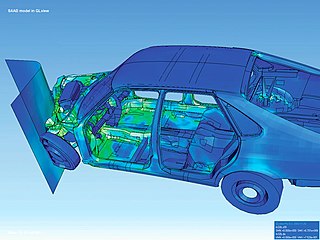
The finite element method (FEM) is an extremely popular method for numerically solving differential equations arising in engineering and mathematical modeling. Typical problem areas of interest include the traditional fields of structural analysis, heat transfer, fluid flow, mass transport, and electromagnetic potential.
In numerical analysis, coarse problem is an auxiliary system of equations used in an iterative method for the solution of a given larger system of equations. A coarse problem is basically a version of the same problem at a lower resolution, retaining its essential characteristics, but with fewer variables. The purpose of the coarse problem is to propagate information throughout the whole problem globally.
The Petrov–Galerkin method is a mathematical method used to approximate solutions of partial differential equations which contain terms with odd order and where the test function and solution function belong to different function spaces. It can be viewed as an extension of Bubnov-Galerkin method where the bases of test functions and solution functions are the same. In an operator formulation of the differential equation, Petrov–Galerkin method can be viewed as applying a projection that is not necessarily orthogonal, in contrast to Bubnov-Galerkin method.
In scientific computation and simulation, the method of fundamental solutions (MFS) is a technique for solving partial differential equations based on using the fundamental solution as a basis function. The MFS was developed to overcome the major drawbacks in the boundary element method (BEM) which also uses the fundamental solution to satisfy the governing equation. Consequently, both the MFS and the BEM are of a boundary discretization numerical technique and reduce the computational complexity by one dimensionality and have particular edge over the domain-type numerical techniques such as the finite element and finite volume methods on the solution of infinite domain, thin-walled structures, and inverse problems.
The Kansa method is a computer method used to solve partial differential equations. Its main advantage is it is very easy to understand and program on a computer. It is much less complicated than the finite element method. Another advantage is it works well on multi variable problems. The finite element method is complicated when working with more than 3 space variables and time.
Fluid motion is governed by the Navier–Stokes equations, a set of coupled and nonlinear partial differential equations derived from the basic laws of conservation of mass, momentum and energy. The unknowns are usually the flow velocity, the pressure and density and temperature. The analytical solution of this equation is impossible hence scientists resort to laboratory experiments in such situations. The answers delivered are, however, usually qualitatively different since dynamical and geometric similitude are difficult to enforce simultaneously between the lab experiment and the prototype. Furthermore, the design and construction of these experiments can be difficult, particularly for stratified rotating flows. Computational fluid dynamics (CFD) is an additional tool in the arsenal of scientists. In its early days CFD was often controversial, as it involved additional approximation to the governing equations and raised additional (legitimate) issues. Nowadays CFD is an established discipline alongside theoretical and experimental methods. This position is in large part due to the exponential growth of computer power which has allowed us to tackle ever larger and more complex problems.
The generalized-strain mesh-free (GSMF) formulation is a local meshfree method in the field of numerical analysis, completely integration free, working as a weighted-residual weak-form collocation. This method was first presented by Oliveira and Portela (2016), in order to further improve the computational efficiency of meshfree methods in numerical analysis. Local meshfree methods are derived through a weighted-residual formulation which leads to a local weak form that is the well known work theorem of the theory of structures. In an arbitrary local region, the work theorem establishes an energy relationship between a statically-admissible stress field and an independent kinematically-admissible strain field. Based on the independence of these two fields, this formulation results in a local form of the work theorem that is reduced to regular boundary terms only, integration-free and free of volumetric locking.

The method of moments (MoM), also known as the moment method and method of weighted residuals, is a numerical method in computational electromagnetics. It is used in computer programs that simulate the interaction of electromagnetic fields such as radio waves with matter, for example antenna simulation programs like NEC that calculate the radiation pattern of an antenna. Generally being a frequency-domain method, it involves the projection of an integral equation into a system of linear equations by the application of appropriate boundary conditions. This is done by using discrete meshes as in finite difference and finite element methods, often for the surface. The solutions are represented with the linear combination of pre-defined basis functions; generally, the coefficients of these basis functions are the sought unknowns. Green's functions and Galerkin method play a central role in the method of moments.

