In computer science, a B-tree is a self-balancing tree data structure that maintains sorted data and allows searches, sequential access, insertions, and deletions in logarithmic time. The B-tree generalizes the binary search tree, allowing for nodes with more than two children. Unlike other self-balancing binary search trees, the B-tree is well suited for storage systems that read and write relatively large blocks of data, such as databases and file systems.

In computer science, a heap is a tree-based data structure that satisfies the heap property: In a max heap, for any given node C, if P is a parent node of C, then the key of P is greater than or equal to the key of C. In a min heap, the key of P is less than or equal to the key of C. The node at the "top" of the heap is called the root node.
In computer science, a linked list is a linear collection of data elements whose order is not given by their physical placement in memory. Instead, each element points to the next. It is a data structure consisting of a collection of nodes which together represent a sequence. In its most basic form, each node contains data, and a reference to the next node in the sequence. This structure allows for efficient insertion or removal of elements from any position in the sequence during iteration. More complex variants add additional links, allowing more efficient insertion or removal of nodes at arbitrary positions. A drawback of linked lists is that data access time is linear in respect to the number of nodes in the list. Because nodes are serially linked, accessing any node requires that the prior node be accessed beforehand. Faster access, such as random access, is not feasible. Arrays have better cache locality compared to linked lists.
In computer science, a priority queue is an abstract data-type similar to a regular queue or stack data structure. Each element in a priority queue has an associated priority. In a priority queue, elements with high priority are served before elements with low priority. In some implementations, if two elements have the same priority, they are served in the same order in which they were enqueued. In other implementations, the order of elements with the same priority is undefined.
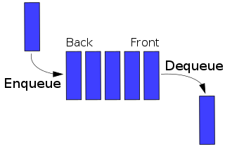
In computer science, a queue is a collection of entities that are maintained in a sequence and can be modified by the addition of entities at one end of the sequence and the removal of entities from the other end of the sequence. By convention, the end of the sequence at which elements are added is called the back, tail, or rear of the queue, and the end at which elements are removed is called the head or front of the queue, analogously to the words used when people line up to wait for goods or services.
In computer science, a red–black tree is a specialised binary search tree data structure noted for fast storage and retrieval of ordered information, and a guarantee that operations will complete within a known time. Compared to other self-balancing binary search trees, the nodes in a red-black tree hold an extra bit called "color" representing "red" and "black" which is used when re-organising the tree to ensure that it is always approximately balanced.
A splay tree is a binary search tree with the additional property that recently accessed elements are quick to access again. Like self-balancing binary search trees, a splay tree performs basic operations such as insertion, look-up and removal in O(log n) amortized time. For random access patterns drawn from a non-uniform random distribution, their amortized time can be faster than logarithmic, proportional to the entropy of the access pattern. For many patterns of non-random operations, also, splay trees can take better than logarithmic time, without requiring advance knowledge of the pattern. According to the unproven dynamic optimality conjecture, their performance on all access patterns is within a constant factor of the best possible performance that could be achieved by any other self-adjusting binary search tree, even one selected to fit that pattern. The splay tree was invented by Daniel Sleator and Robert Tarjan in 1985.

A binary heap is a heap data structure that takes the form of a binary tree. Binary heaps are a common way of implementing priority queues. The binary heap was introduced by J. W. J. Williams in 1964, as a data structure for heapsort.
In computer science, a binomial heap is a data structure that acts as a priority queue. It is an example of a mergeable heap, as it supports merging two heaps in logarithmic time. It is implemented as a heap similar to a binary heap but using a special tree structure that is different from the complete binary trees used by binary heaps. Binomial heaps were invented in 1978 by Jean Vuillemin.
In computer science, a Fibonacci heap is a data structure for priority queue operations. It has a better amortized running time than many other priority queue data structures including the binary heap and binomial heap. consisting of a collection of heap-ordered trees. Fibonacci heaps were originally explained to be an extension of binomial heaps. Michael L. Fredman and Robert E. Tarjan developed Fibonacci heaps in 1984 and published them in a scientific journal in 1987. Fibonacci heaps are named after the Fibonacci numbers, which are used in their running time analysis.
In computing, a persistent data structure or not ephemeral data structure is a data structure that always preserves the previous version of itself when it is modified. Such data structures are effectively immutable, as their operations do not (visibly) update the structure in-place, but instead always yield a new updated structure. The term was introduced in Driscoll, Sarnak, Sleator, and Tarjan's 1986 article.
In computer science, a 2–3 heap is a data structure, a variation on the heap, designed by Tadao Takaoka in 1999. The structure is similar to the Fibonacci heap, and borrows from the 2–3 tree.
In computer science, a disjoint-set data structure, also called a union–find data structure or merge–find set, is a data structure that stores a collection of disjoint (non-overlapping) sets. Equivalently, it stores a partition of a set into disjoint subsets. It provides operations for adding new sets, merging sets, and finding a representative member of a set. The last operation makes it possible to find out efficiently if any two elements are in the same or different sets.
A van Emde Boas tree, also known as a vEB tree or van Emde Boas priority queue, is a tree data structure which implements an associative array with m-bit integer keys. It was invented by a team led by Dutch computer scientist Peter van Emde Boas in 1975. It performs all operations in O(log m) time, or equivalently in time, where is the largest element that can be stored in the tree. The parameter is not to be confused with the actual number of elements stored in the tree, by which the performance of other tree data-structures is often measured.
A B+ tree is an m-ary tree with a variable but often large number of children per node. A B+ tree consists of a root, internal nodes and leaves. The root may be either a leaf or a node with two or more children.
A pairing heap is a type of heap data structure with relatively simple implementation and excellent practical amortized performance, introduced by Michael Fredman, Robert Sedgewick, Daniel Sleator, and Robert Tarjan in 1986. Pairing heaps are heap-ordered multiway tree structures, and can be considered simplified Fibonacci heaps. They are considered a "robust choice" for implementing such algorithms as Prim's MST algorithm, and support the following operations :
In computer science, a skew binomial heap is a variant of the binomial heap that supports constant-time insertion operations in the worst case, rather than the logarithmic worst case and constant amortized time of ordinary binomial heaps.
In computer science, Iacono's working set structure is a comparison based dictionary. It supports insertion, deletion and access operation to maintain a dynamic set of elements. The working set of an item is the set of elements that have been accessed in the structure since the last time that was accessed . Inserting and deleting in the working set structure takes time while accessing an element takes . Here, represents the size of the working set of .
In computer science, the order-maintenance problem involves maintaining a totally ordered set supporting the following operations:
In computer science, a shadow heap is a mergeable heap data structure which supports efficient heap merging in the amortized sense. More specifically, shadow heaps make use of the shadow merge algorithm to achieve insertion in O(f(n)) amortized time and deletion in O((log n log log n)/f(n)) amortized time, for any choice of 1 ≤ f(n) ≤ log log n.