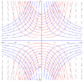
Slope field

Last updated
The slope field of
d
y
d
x
=
x
2
-
x
-
2
{\displaystyle {\frac {dy}{dx}}=x^{2}-x-2}
, with the blue, red, and turquoise lines being
x
3
3
-
x
2
2
-
2
x
+
4
{\displaystyle {\frac {x^{3}}{3}}-{\frac {x^{2}}{2}}-2x+4}
,
x
3
3
-
x
2
2
-
2
x
{\displaystyle {\frac {x^{3}}{3}}-{\frac {x^{2}}{2}}-2x}
, and
x
3
3
-
x
2
2
-
2
x
-
4
{\displaystyle {\frac {x^{3}}{3}}-{\frac {x^{2}}{2}}-2x-4}
, respectively. Slope Field.png
The slope field of , with the blue, red, and turquoise lines being , , and , respectively.

Slope fields (also called direction fields [1] ) are a graphical representation of the solutions to a first-order differential equation [2] of a scalar function. Solutions to a slope field are functions drawn as solid curves. A slope field shows the slope of a differential equation at certain vertical and horizontal intervals on the x-y plane, and can be used to determine the approximate tangent slope at a point on a curve, where the curve is some solution to the differential equation.

Contents

Definition

Standard case

The slope field can be defined for the following type of differential equations

which can be interpreted geometrically as giving the slope of the tangent to the graph of the differential equation's solution ( integral curve ) at each point (x, y) as a function of the point coordinates. [3]

It can be viewed as a creative way to plot a real-valued function of two real variables as a planar picture. Specifically, for a given pair , a vector with the components is drawn at the point on the -plane. Sometimes, the vector is normalized to make the plot better looking for a human eye. A set of pairs making a rectangular grid is typically used for the drawing.

An isocline (a series of lines with the same slope) is often used to supplement the slope field. In an equation of the form , the isocline is a line in the -plane obtained by setting equal to a constant.

General case of a system of differential equations

Given a system of differential equations,

the slope field is an array of slope marks in the phase space (in any number of dimensions depending on the number of relevant variables; for example, two in the case of a first-order linear ODE, as seen to the right). Each slope mark is centered at a point and is parallel to the vector

The number, position, and length of the slope marks can be arbitrary. The positions are usually chosen such that the points make a uniform grid. The standard case, described above, represents . The general case of the slope field for systems of differential equations is not easy to visualize for .

General application

With computers, complicated slope fields can be quickly made without tedium, and so an only recently practical application is to use them merely to get the feel for what a solution should be before an explicit general solution is sought. Of course, computers can also just solve for one, if it exists.

If there is no explicit general solution, computers can use slope fields (even if they aren’t shown) to numerically find graphical solutions. Examples of such routines are Euler's method, or better, the Runge–Kutta methods.

Software for plotting slope fields

Different software packages can plot slope fields.

Direction field code in GNU Octave/MATLAB

funn=@(x,y)y-x;% function f(x, y) = y-x[x,y]=meshgrid(-5:0.5:5);% intervals for x and yslopes=funn(x,y);% matrix of slope valuesdy=slopes./sqrt(1+slopes.^2);% normalize the line element...dx=ones(length(dy))./sqrt(1+slopes.^2);% ...magnitudes for dy and dxh=quiver(x,y,dx,dy,0.5);% plot the direction fieldset(h,"maxheadsize",0.1);% alter head size

Example code for Maxima

/* field for y'=xy (click on a point to get an integral curve). Plotdf requires Xmaxima  */ plotdf( x*y, [x,-2,2], [y,-2,2]);

Example code for Mathematica

(* field for y'=xy *)VectorPlot[{1,x*y-5x},{x,-2,2},{y,-2,2}]

Example code for SageMath [4]

var('x,y') plot_slope_field(x*y, (x,-2,2), (y,-2,2)) 

Examples

See also

Related Research Articles

<span class="mw-page-title-main">Derivative</span> Instantaneous rate of change (mathematics)

In mathematics, the derivative shows the sensitivity of change of a function's output with respect to the input. Derivatives are a fundamental tool of calculus. For example, the derivative of the position of a moving object with respect to time is the object's velocity: this measures how quickly the position of the object changes when time advances.

<span class="mw-page-title-main">Tangent</span> In mathematics, straight line touching a plane curve without crossing it

In geometry, the tangent line (or simply tangent) to a plane curve at a given point is the straight line that "just touches" the curve at that point. Leibniz defined it as the line through a pair of infinitely close points on the curve. More precisely, a straight line is said to be a tangent of a curve y = f(x) at a point x = c if the line passes through the point (c, f(c)) on the curve and has slope f'(c), where f' is the derivative of f. A similar definition applies to space curves and curves in n-dimensional Euclidean space.

<span class="mw-page-title-main">Differential calculus</span> Area of mathematics; subarea of calculus

In mathematics, differential calculus is a subfield of calculus that studies the rates at which quantities change. It is one of the two traditional divisions of calculus, the other being integral calculus—the study of the area beneath a curve.

<span class="mw-page-title-main">Calculus of variations</span> Differential calculus on function spaces

The calculus of variations is a field of mathematical analysis that uses variations, which are small changes in functions and functionals, to find maxima and minima of functionals: mappings from a set of functions to the real numbers. Functionals are often expressed as definite integrals involving functions and their derivatives. Functions that maximize or minimize functionals may be found using the Euler–Lagrange equation of the calculus of variations.

In mathematics, differential forms provide a unified approach to define integrands over curves, surfaces, solids, and higher-dimensional manifolds. The modern notion of differential forms was pioneered by Élie Cartan. It has many applications, especially in geometry, topology and physics.

<span class="mw-page-title-main">Green's theorem</span> Theorem in calculus relating line and double integrals

In vector calculus, Green's theorem relates a line integral around a simple closed curve C to a double integral over the plane region D bounded by C. It is the two-dimensional special case of Stokes' theorem.

<span class="mw-page-title-main">Implicit function</span> Mathematical relation consisting of a multi-variable function equal to zero

In mathematics, an implicit equation is a relation of the form where R is a function of several variables. For example, the implicit equation of the unit circle is

In mathematics, the Hodge star operator or Hodge star is a linear map defined on the exterior algebra of a finite-dimensional oriented vector space endowed with a nondegenerate symmetric bilinear form. Applying the operator to an element of the algebra produces the Hodge dual of the element. This map was introduced by W. V. D. Hodge.

<span class="mw-page-title-main">Autonomous system (mathematics)</span> System of ordinary differential equations whose current state solely determines its evolution

In mathematics, an autonomous system or autonomous differential equation is a system of ordinary differential equations which does not explicitly depend on the independent variable. When the variable is time, they are also called time-invariant systems.

Hilbert's 16th problem was posed by David Hilbert at the Paris conference of the International Congress of Mathematicians in 1900, as part of his list of 23 problems in mathematics.

<span class="mw-page-title-main">Euler equations (fluid dynamics)</span> Set of quasilinear hyperbolic equations governing adiabatic and inviscid flow

In fluid dynamics, the Euler equations are a set of quasilinear partial differential equations governing adiabatic and inviscid flow. They are named after Leonhard Euler. In particular, they correspond to the Navier–Stokes equations with zero viscosity and zero thermal conductivity.

<span class="mw-page-title-main">Total derivative</span> Type of derivative in mathematics

In mathematics, the total derivative of a function f at a point is the best linear approximation near this point of the function with respect to its arguments. Unlike partial derivatives, the total derivative approximates the function with respect to all of its arguments, not just a single one. In many situations, this is the same as considering all partial derivatives simultaneously. The term "total derivative" is primarily used when f is a function of several variables, because when f is a function of a single variable, the total derivative is the same as the ordinary derivative of the function.

In mathematical analysis, and applications in geometry, applied mathematics, engineering, and natural sciences, a function of a real variable is a function whose domain is the real numbers , or a subset of that contains an interval of positive length. Most real functions that are considered and studied are differentiable in some interval. The most widely considered such functions are the real functions, which are the real-valued functions of a real variable, that is, the functions of a real variable whose codomain is the set of real numbers.

In mathematics, an integral curve is a parametric curve that represents a specific solution to an ordinary differential equation or system of equations.

<span class="mw-page-title-main">Differential equation</span> Type of functional equation (mathematics)

In mathematics, a differential equation is an equation that relates one or more unknown functions and their derivatives. In applications, the functions generally represent physical quantities, the derivatives represent their rates of change, and the differential equation defines a relationship between the two. Such relations are common; therefore, differential equations play a prominent role in many disciplines including engineering, physics, economics, and biology.

In mathematics, an integrating factor is a function that is chosen to facilitate the solving of a given equation involving differentials. It is commonly used to solve ordinary differential equations, but is also used within multivariable calculus when multiplying through by an integrating factor allows an inexact differential to be made into an exact differential. This is especially useful in thermodynamics where temperature becomes the integrating factor that makes entropy an exact differential.

In applied mathematics, in particular the context of nonlinear system analysis, a phase plane is a visual display of certain characteristics of certain kinds of differential equations; a coordinate plane with axes being the values of the two state variables, say (x, y), or (q, p) etc. (any pair of variables). It is a two-dimensional case of the general n-dimensional phase space.

<span class="mw-page-title-main">Notation for differentiation</span> Notation of differential calculus

In differential calculus, there is no single uniform notation for differentiation. Instead, various notations for the derivative of a function or variable have been proposed by various mathematicians. The usefulness of each notation varies with the context, and it is sometimes advantageous to use more than one notation in a given context. The most common notations for differentiation are listed below.

<span class="mw-page-title-main">Differential of a function</span> Notion in calculus

In calculus, the differential represents the principal part of the change in a function with respect to changes in the independent variable. The differential is defined by

In mathematical analysis and its applications, a function of several real variables or real multivariate function is a function with more than one argument, with all arguments being real variables. This concept extends the idea of a function of a real variable to several variables. The "input" variables take real values, while the "output", also called the "value of the function", may be real or complex. However, the study of the complex-valued functions may be easily reduced to the study of the real-valued functions, by considering the real and imaginary parts of the complex function; therefore, unless explicitly specified, only real-valued functions will be considered in this article.

References

  1. Boyce, William (2001). Elementary differential equations and boundary value problems (7 ed.). Wiley. p. 3. ISBN   9780471319993.
  2. Vladimir A. Dobrushkin (2014). Applied Differential Equations: The Primary Course. CRC Press. p. 13. ISBN   978-1-4987-2835-5.
  3. Andrei D. Polyanin; Alexander V. Manzhirov (2006). Handbook of Mathematics for Engineers and Scientists. CRC Press. p. 453. ISBN   978-1-58488-502-3.
  4. "Plotting fields — Sage 9.4 Reference Manual: 2D Graphics".