Standard step method

Last updated

The standard step method (STM) is a computational technique utilized to estimate one-dimensional surface water profiles in open channels with gradually varied flow under steady state conditions. It uses a combination of the energy, momentum, and continuity equations to determine water depth with a given a friction slope , channel slope , channel geometry, and also a given flow rate. In practice, this technique is widely used through the computer program HEC-RAS, developed by the US Army Corps of Engineers Hydrologic Engineering Center (HEC). [1]

Contents

Open channel flow fundamentals

Figure 1. Conceptual figure used to define terms in the energy equation. Open Channel Flow Energy Lines.jpg
Figure 1. Conceptual figure used to define terms in the energy equation.
Figure 2. A diagram showing the relationship for flow depth (y) and total Energy (E) for a given flow (Q). Note the location of critical flow, subcritical flow, and supercritical flow. E-y Diagram.jpg
Figure 2. A diagram showing the relationship for flow depth (y) and total Energy (E) for a given flow (Q). Note the location of critical flow, subcritical flow, and supercritical flow.

The energy equation used for open channel flow computations is a simplification of the Bernoulli Equation (See Bernoulli Principle), which takes into account pressure head, elevation head, and velocity head. (Note, energy and head are synonymous in Fluid Dynamics. See Pressure head for more details.) In open channels, it is assumed that changes in atmospheric pressure are negligible, therefore the “pressure head” term used in Bernoulli’s Equation is eliminated. The resulting energy equation is shown below:

          Equation 1

For a given flow rate and channel geometry, there is a relationship between flow depth and total energy. This is illustrated below in the plot of energy vs. flow depth, widely known as an E-y diagram. In this plot, the depth where the minimum energy occurs is known as the critical depth. Consequently, this depth corresponds to a Froude Number of 1. Depths greater than critical depth are considered “subcritical” and have a Froude Number less than 1, while depths less than critical depth are considered supercritical and have Froude Numbers greater than 1.

          Equation 2

Under steady state flow conditions (e.g. no flood wave), open channel flow can be subdivided into three types of flow: uniform flow, gradually varying flow, and rapidly varying flow. Uniform flow describes a situation where flow depth does not change with distance along the channel. This can only occur in a smooth channel that does not experience any changes in flow, channel geometry, roughness or channel slope. During uniform flow, the flow depth is known as normal depth (yn). This depth is analogous to the terminal velocity of an object in free fall, where gravity and frictional forces are in balance (Moglen, 2013). [3] Typically, this depth is calculated using the Manning formula. Gradually varied flow occurs when the change in flow depth per change in flow distance is very small. In this case, hydrostatic relationships developed for uniform flow still apply. Examples of this include the backwater behind an in-stream structure (e.g. dam, sluice gate, weir, etc.), when there is a constriction in the channel, and when there is a minor change in channel slope. Rapidly varied flow occurs when the change in flow depth per change in flow distance is significant. In this case, hydrostatics relationships are not appropriate for analytical solutions, and continuity of momentum must be employed. Examples of this include large changes in slope like a spillway, abrupt constriction/expansion of flow, or a hydraulic jump.

Water surface profiles (gradually varied flow)

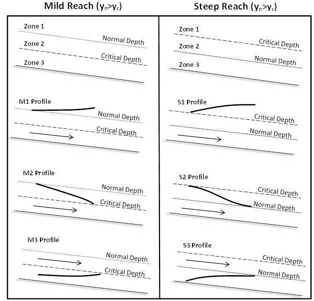
Typically, the STM is used to develop “surface water profiles,” or longitudinal representations of channel depth, for channels experiencing gradually varied flow. These transitions can be classified based on reach condition (mild or steep), and also the type of transition being made. Mild reaches occur where normal depth is subcritical (yn > yc) while steep reaches occur where normal depth is supercritical (yn<yc). The transitions are classified by zone. (See figure 3.)

Surface Water Profiles.jpg

Figure 3. This figure illustrates the different classes of surface water profiles experienced in steep and mild reaches during gradually varied flow conditions. [4] Note: The Steep Reach column should be labeled "Steep Reach (yn<yc).

The above surface water profiles are based on the governing equation for gradually varied flow (seen below)

          Equation 3

This equation (and associated surface water profiles) is based on the following assumptions:

  • The slope is relatively small
  • Channel cross-section is known at stations of interest
  • There is a hydrostatic pressure distribution

Standard step method calculation

The STM numerically solves equation 3 through an iterative process. This can be done using the bisection or Newton-Raphson Method, and is essentially solving for total head at a specified location using equations 4 and 5 by varying depth at the specified location. [5]

          Equation 4
          Equation 5

In order to use this technique, it is important to note you must have some understanding of the system you are modeling. For each gradually varied flow transition, you must know both boundary conditions and you must also calculate length of that transition. (e.g. For an M1 Profile, you must find the rise at the downstream boundary condition, the normal depth at the upstream boundary condition, and also the length of the transition.) To find the length of the gradually varied flow transitions, iterate the “step length”, instead of height, at the boundary condition height until equations 4 and 5 agree. (e.g. For an M1 Profile, position 1 would be the downstream condition and you would solve for position two where the height is equal to normal depth.)

Newton–Raphson numerical method

NewtonRaphsonMethod.jpg

Computer programs like excel contain iteration or goal seek functions that can automatically calculate the actual depth instead of manual iteration.

Conceptual surface water profiles (sluice gate)

Figure 4. Illustration of surface water profiles associated with a sluice gate in a mild reach (top) and a steep reach (bottom). Sluice Gate Sketch.jpg
Figure 4. Illustration of surface water profiles associated with a sluice gate in a mild reach (top) and a steep reach (bottom).

Figure 4 illustrates the different surface water profiles associated with a sluice gate on a mild reach (top) and a steep reach (bottom). Note, the sluice gate induces a choke in the system, causing a “backwater” profile just upstream of the gate. In the mild reach, the hydraulic jump occurs downstream of the gate, but in the steep reach, the hydraulic jump occurs upstream of the gate. It is important to note that the gradually varied flow equations and associated numerical methods (including the standard step method) cannot accurately model the dynamics of a hydraulic jump. [6] See the Hydraulic jumps in rectangular channels page for more information. Below, an example problem will use conceptual models to build a surface water profile using the STM.

Example problem

Large Standard Step Method Problem Statement.jpg

Solution

Large Standard Step Method Step 1.jpg


Large Standart Step Method Step 2 drawing.jpg


Large Standard Step Method Step 3.jpg


Using Figure 3 and knowledge of the upstream and downstream conditions and the depth values on either side of the gate, a general estimate of the profiles upstream and downstream of the gate can be generated. Upstream, the water surface must rise from a normal depth of 0.97 m to 9.21 m at the gate. The only way to do this on a mild reach is to follow an M1 profile. The same logic applies downstream to determine that the water surface follows an M3 profile from the gate until the depth reaches the conjugate depth of the normal depth at which point a hydraulic jump forms to raise the water surface to the normal depth.

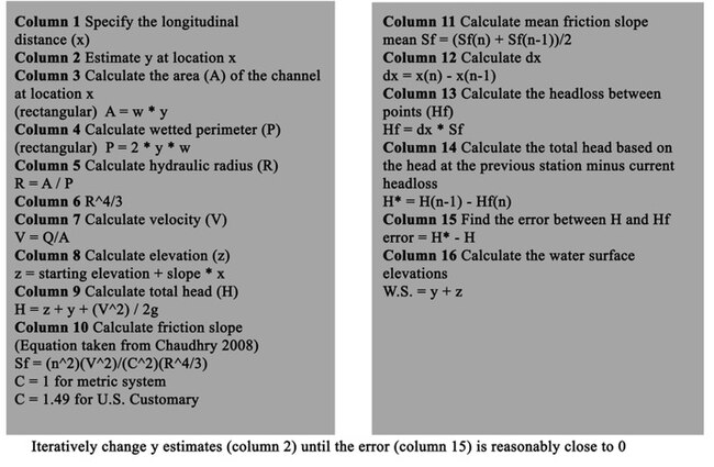
Step 4: Use the Newton Raphson Method to solve the M1 and M3 surface water profiles. The upstream and downstream portions must be modeled separately with an initial depth of 9.21 m for the upstream portion, and 0.15 m for the downstream portion. The downstream depth should only be modeled until it reaches the conjugate depth of the normal depth, at which point a hydraulic jump will form. The solution presented explains how to solve the problem in a spreadsheet, showing the calculations column by column. Within Excel, the goal seek function can be used to set column 15 to 0 by changing the depth estimate in column 2 instead of iterating manually.


Large Standard Step Method Step 4.jpg

Large Standard Step Spreadsheet.jpg

Table 1: Spreadsheet of Newton Raphson Method of downstream water surface elevation calculations


Step 5: Combine the results from the different profiles and display.

Upstream Water Surface Profile.jpg

Downstream Water Surface Profile.jpg

Normal depth was achieved at approximately 2,200 meters upstream of the gate.

Step 6: Solve the problem in the HEC-RAS Modeling Environment:

It is beyond the scope of this Wikipedia Page to explain the intricacies of operating HEC-RAS. For those interested in learning more, the HEC-RAS user’s manual is an excellent learning tool and the program is free to the public.

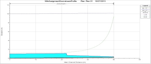
The first two figures below are the upstream and downstream water surface profiles modeled by HEC-RAS. There is also a table provided comparing the differences between the profiles estimated by the two different methods at different stations to show consistency between the two methods. While the two different methods modeled similar water surface shapes, the standard step method predicted that the flow would take a greater distance to reach normal depth upstream and downstream of the gate. This stretching is caused by the errors associated with assuming average gradients between two stations of interest during our calculations. Smaller dx values would reduce this error and produce more accurate surface profiles.

HEC-RAS Modle Upstream gate.jpg

HEC-RAS model Downstream of gate with jump.jpg

The HEC-RAS model calculated that the water backs up to a height of 9.21 meters at the upstream side of the sluice gate, which is the same as the manually calculated value. Normal depth was achieved at approximately 1,700 meters upstream of the gate.

HEC-RAS modeled the hydraulic jump to occur 18 meters downstream of the sluice gate.

Large Standard Step Comparison Table.jpg

Related Research Articles

<span class="mw-page-title-main">Hydraulic jump</span> Discharge of high velocity liquid into lower velocity area

A hydraulic jump is a phenomenon in the science of hydraulics which is frequently observed in open channel flow such as rivers and spillways. When liquid at high velocity discharges into a zone of lower velocity, a rather abrupt rise occurs in the liquid surface. The rapidly flowing liquid is abruptly slowed and increases in height, converting some of the flow's initial kinetic energy into an increase in potential energy, with some energy irreversibly lost through turbulence to heat. In an open channel flow, this manifests as the fast flow rapidly slowing and piling up on top of itself similar to how a shockwave forms.

<span class="mw-page-title-main">Weir</span> Artificial river barrier

A weir or low head dam is a barrier across the width of a river that alters the flow characteristics of water and usually results in a change in the height of the river level. Weirs are also used to control the flow of water for outlets of lakes, ponds, and reservoirs. There are many weir designs, but commonly water flows freely over the top of the weir crest before cascading down to a lower level.

<span class="mw-page-title-main">Sluice</span> Water channel controlled at its head by a gate

Sluice is a word for a channel controlled at its head by a movable gate which is called a sluice gate. A sluice gate is traditionally a wood or metal barrier sliding in grooves that are set in the sides of the waterway and can be considered as a bottom opening in a wall. Sluice gates are one of the most common hydraulic structures in controlling flow rate and water level in open channels such as rivers and canals. They also could be used to measure the flow. A water channel containing a sluice gate forms a type of lock to manage the water flow and water level. It can also be an open channel which processes material, such as a River Sluice used in gold prospecting or fossicking. A mill race, leet, flume, penstock or lade is a sluice channeling water toward a water mill. The terms sluice, sluice gate, knife gate, and slide gate are used interchangeably in the water and wastewater control industry. They are also used in wastewater treatment plants and to recover minerals in mining operations, and in watermills.

<span class="mw-page-title-main">Hydraulic head</span> Specific measurement of liquid pressure above a vertical datum

Hydraulic head or piezometric head is a specific measurement of liquid pressure above a vertical datum.

<span class="mw-page-title-main">Open-channel flow</span> Type of liquid flow within a conduit

In fluid mechanics and hydraulics, open-channel flow is a type of liquid flow within a conduit with a free surface, known as a channel. The other type of flow within a conduit is pipe flow. These two types of flow are similar in many ways but differ in one important respect: open-channel flow has a free surface, whereas pipe flow does not.

<span class="mw-page-title-main">HEC-RAS</span>

HEC-RAS is a computer program that models the hydraulics of water flow through natural rivers and other channels. Prior to the 2016 update to Version 5.0, the program was one-dimensional, meaning that there is no direct modeling of the hydraulic effect of cross section shape changes, bends, and other two- and three-dimensional aspects of flow. The release of Version 5.0 introduced two-dimensional modeling of flow as well as sediment transfer modeling capabilities. The program was developed by the United States Army Corps of Engineers in order to manage the rivers, harbors, and other public works under their jurisdiction; it has found wide acceptance by many others since its public release in 1995.

<span class="mw-page-title-main">Sediment transport</span> Movement of solid particles, typically by gravity and fluid entrainment

Sediment transport is the movement of solid particles (sediment), typically due to a combination of gravity acting on the sediment, and/or the movement of the fluid in which the sediment is entrained. Sediment transport occurs in natural systems where the particles are clastic rocks, mud, or clay; the fluid is air, water, or ice; and the force of gravity acts to move the particles along the sloping surface on which they are resting. Sediment transport due to fluid motion occurs in rivers, oceans, lakes, seas, and other bodies of water due to currents and tides. Transport is also caused by glaciers as they flow, and on terrestrial surfaces under the influence of wind. Sediment transport due only to gravity can occur on sloping surfaces in general, including hillslopes, scarps, cliffs, and the continental shelf—continental slope boundary.

<span class="mw-page-title-main">Shallow water equations</span> Set of partial differential equations that describe the flow below a pressure surface in a fluid

The shallow-water equations are a set of hyperbolic partial differential equations that describe the flow below a pressure surface in a fluid. The shallow-water equations in unidirectional form are also called Saint-Venant equations, after Adhémar Jean Claude Barré de Saint-Venant.

The Chézy formula is an semi-empirical resistance equation which estimates mean flow velocity in open channel conduits. The relationship was realized and developed in 1768 by French physicist and engineer Antoine de Chézy (1718–1798) while designing Paris's water canal system. Chézy discovered a similarity parameter that could be used for estimating flow characteristics in one channel based on the measurements of another. The Chézy formula relates the flow of water through an open channel with the channel's dimensions and slope. The Chézy equation is a pioneering formula in the field of fluid mechanics and was expanded and modified by Irish Engineer Robert Manning in 1889. Manning's modifications to the Chézy formula allowed the entire similarity parameter to be calculated by channel characteristics rather than by experimental measurements. Today, the Chézy and Manning equations continue to accurately estimate open channel fluid flow and are standard formulas in all fields that relate to fluid mechanics and hydraulics, including physics, mechanical engineering and civil engineering.

<span class="mw-page-title-main">Bridge scour</span> Removal of sediment from around bridge abutments or piers by the movement of water

Bridge scour is the removal of sediment such as sand and gravel from around bridge abutments or piers. Hydrodynamic scour, caused by fast flowing water, can carve out scour holes, compromising the integrity of a structure.

Hydraulic jump in a rectangular channel, also known as classical jump, is a natural phenomenon that occurs whenever flow changes from supercritical to subcritical flow. In this transition, the water surface rises abruptly, surface rollers are formed, intense mixing occurs, air is entrained, and often a large amount of energy is dissipated. Numeric models created using the standard step method or HEC-RAS are used to track supercritical and subcritical flows to determine where in a specific reach a hydraulic jump will form.

In open channel flow, specific energy (e) is the energy length, or head, relative to the channel bottom. Specific energy is expressed in terms of kinetic energy, and potential energy, and internal energy. The Bernoulli equation, which originates from a control volume analysis, is used to describe specific energy relationships in fluid dynamics. The form of Bernoulli’s equation discussed here assumes the flow is incompressible and steady. The three energy components in Bernoulli's equation are elevation, pressure and velocity. However, since with open channel flow, the water surface is open to the atmosphere, the pressure term between two points has the same value and is therefore ignored. Thus, if the specific energy and the velocity of the flow in the channel are known, the depth of flow can be determined. This relationship can be used to calculate changes in depth upstream or downstream of changes in the channel such as steps, constrictions, or control structures. It is also the fundamental relationship used in the standard step method to calculate how the depth of a flow changes over a reach from the energy gained or lost due to the slope of the channel.

<span class="mw-page-title-main">Dimensionless specific energy diagrams for open-channel flow</span>

Energy conservation is an important concept when analyzing open channel flows. For the purposes of the following analysis, energy is conserved for a fluid in an open channel flow, and head losses due to friction will be neglected. The energy calculated at one location in the flow will be equal to the energy calculated at any other location in the same flow.

In classical physics, momentum is the product of mass and velocity and is a vector quantity, but in fluid mechanics it is treated as a longitudinal quantity evaluated in the direction of flow. Additionally, it is evaluated as momentum per unit time, corresponding to the product of mass flow rate and velocity, and therefore it has units of force. The momentum forces considered in open channel flow are dynamic force – dependent of depth and flow rate – and static force – dependent of depth – both affected by gravity.

In gravity and pressure driven fluid dynamical and geophysical mass flows such as ocean waves, avalanches, debris flows, mud flows, flash floods, etc., kinematic waves are important mathematical tools to understand the basic features of the associated wave phenomena. These waves are also applied to model the motion of highway traffic flows.

In hydrology, routing is a technique used to predict the changes in shape of a hydrograph as water moves through a river channel or a reservoir. In flood forecasting, hydrologists may want to know how a short burst of intense rain in an area upstream of a city will change as it reaches the city. Routing can be used to determine whether the pulse of rain reaches the city as a deluge or a trickle.

<span class="mw-page-title-main">Parshall flume</span> Hydraulic structure for measuring fluid flow

The Parshall flume is an open channel flow metering device that was developed to measure the flow of surface waters and irrigation flows. The Parshall flume is a fixed hydraulic structure. It is used to measure volumetric flow rate in industrial discharges, municipal sewer lines, and influent/effluent flows in wastewater treatment plants. The Parshall flume accelerates flow through a contraction of both the parallel sidewalls and a drop in the floor at the flume throat. Under free-flow conditions the depth of water at specified location upstream of the flume throat can be converted to a rate of flow. Some states specify the use of Parshall flumes, by law, for certain situations.

A common open channel flow problem is determining the discharge from a lake to a rectangular channel.

<span class="mw-page-title-main">Open channel spillway</span>

Open channel spillways are dam spillways that utilize the principles of open-channel flow to convey impounded water in order to prevent dam failure. They can function as principal spillways, emergency spillways, or both. They can be located on the dam itself or on a natural grade in the vicinity of the dam.

References

  1. USACE. "HEC-RAS Version 4.1 User's Manual". Hydrologic Engineering Center, Davis, CA.{{cite web}}: Missing or empty |url= (help)
  2. Chaudhry, M.H. (2008). Open-Channel Flow. New York: Springer.
  3. Moglen, G. "Lecture Notes from CEE 4324/5894: Open Channel Flow, Virginia Tech". Archived from the original on November 5, 2012. Retrieved April 24, 2013.
  4. Chow, V.T. (1959). Open-Channel Hydraulics. New York: McGraw-Hill.
  5. Chaudhry, M.H. (2008). Open-Channel Flow. New York: Springer.
  6. Chaudhry, M.H. (2008). Open-Channel Flow. New York: Springer.