In mathematics, the determinant is a scalar value that is a function of the entries of a square matrix. It allows characterizing some properties of the matrix and the linear map represented by the matrix. In particular, the determinant is nonzero if and only if the matrix is invertible and the linear map represented by the matrix is an isomorphism. The determinant of a product of matrices is the product of their determinants . The determinant of a matrix A is denoted det(A), det A, or |A|.

In mathematics, a tensor is an algebraic object that describes a multilinear relationship between sets of algebraic objects related to a vector space. Objects that tensors may map between include vectors and scalars, and even other tensors. There are many types of tensors, including scalars and vectors, dual vectors, multilinear maps between vector spaces, and even some operations such as the dot product. Tensors are defined independent of any basis, although they are often referred to by their components in a basis related to a particular coordinate system.

In geometry, a tetrahedron, also known as a triangular pyramid, is a polyhedron composed of four triangular faces, six straight edges, and four vertex corners. The tetrahedron is the simplest of all the ordinary convex polyhedra and the only one that has fewer than 5 faces.
In mathematics, the tensor product of two vector spaces V and W is a vector space which can be thought of as the space of all tensors that can be built from vectors from its constituent spaces using an additional operation which can be considered as a generalization and abstraction of the outer product. Because of the connection with tensors, which are the elements of a tensor product, tensor products find uses in many areas of application including in physics and engineering, though the full theoretical mechanics of them described below may not be commonly cited there. For example, in general relativity, the gravitational field is described through the metric tensor, which is a field of tensors, one at each point in the space-time manifold, and each of which lives in the tensor self-product of tangent spaces at its point of residence on the manifold.

In mathematics, physics and engineering, a Euclidean vector or simply a vector is a geometric object that has magnitude and direction. Vectors can be added to other vectors according to vector algebra. A Euclidean vector is frequently represented by a ray, or graphically as an arrow connecting an initial pointA with a terminal pointB, and denoted by .
In linear algebra, the trace of a square matrix A, denoted tr(A), is defined to be the sum of elements on the main diagonal of A.

In mathematics, the cross product or vector product is a binary operation on two vectors in three-dimensional space , and is denoted by the symbol . Given two linearly independent vectors a and b, the cross product, a × b, is a vector that is perpendicular to both a and b, and thus normal to the plane containing them. It has many applications in mathematics, physics, engineering, and computer programming. It should not be confused with the dot product.
In mathematics, the dot product or scalar product is an algebraic operation that takes two equal-length sequences of numbers, and returns a single number. In Euclidean geometry, the dot product of the Cartesian coordinates of two vectors is widely used. It is often called "the" inner product of Euclidean space, even though it is not the only inner product that can be defined on Euclidean space.
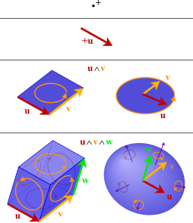
In mathematics, the exterior product or wedge product of vectors is an algebraic construction used in geometry to study areas, volumes, and their higher-dimensional analogues. The exterior product of two vectors and , denoted by , is called a bivector and lives in a space called the exterior square, a vector space that is distinct from the original space of vectors. The magnitude of can be interpreted as the area of the parallelogram with sides and , which in three dimensions can also be computed using the cross product of the two vectors. More generally, all parallel plane surfaces with the same orientation and area have the same bivector as a measure of their oriented area. Like the cross product, the exterior product is anticommutative, meaning that for all vectors and , but, unlike the cross product, the exterior product is associative.
In mathematics, a homogeneous function is one with multiplicative scaling behaviour: if all its arguments are multiplied by a factor, then its value is multiplied by some power of this factor.

In physics, the reciprocal lattice represents the Fourier transform of another lattice. In normal usage, the initial lattice is usually a periodic spatial function in real-space and is also known as the direct lattice. While the direct lattice exists in real-space and is what one would commonly understand as a physical lattice, the reciprocal lattice exists in reciprocal space. The reciprocal lattice of a reciprocal lattice is equivalent to the original direct lattice, because the defining equations are symmetrical with respect to the vectors in real and reciprocal space. Mathematically, direct and reciprocal lattice vectors represent covariant and contravariant vectors, respectively.
In abstract algebra and multilinear algebra, a multilinear form on a vector space over a field is a map
In mathematics, the discrete Laplace operator is an analog of the continuous Laplace operator, defined so that it has meaning on a graph or a discrete grid. For the case of a finite-dimensional graph, the discrete Laplace operator is more commonly called the Laplacian matrix.
In the mathematical field of graph theory, the Laplacian matrix, also called the graph Laplacian, admittance matrix, Kirchhoff matrix or discrete Laplacian, is a matrix representation of a graph. The Laplacian matrix can be used to find many useful properties of a graph. Together with Kirchhoff's theorem, it can be used to calculate the number of spanning trees for a given graph. The sparsest cut of a graph can be approximated through the second smallest eigenvalue of its Laplacian by Cheeger's inequality. It can also be used to construct low dimensional embeddings, which can be useful for a variety of machine learning applications.
In the mathematical discipline of graph theory, the edge space and vertex space of an undirected graph are vector spaces defined in terms of the edge and vertex sets, respectively. These vector spaces make it possible to use techniques of linear algebra in studying the graph.

Three-dimensional space is a geometric setting in which three values are required to determine the position of an element. This is the informal meaning of the term dimension.
In mathematics and physics, a quantum graph is a linear, network-shaped structure of vertices connected on edges in which each edge is given a length and where a differential equation is posed on each edge. An example would be a power network consisting of power lines (edges) connected at transformer stations (vertices); the differential equations would then describe the voltage along each of the lines, with boundary conditions for each edge provided at the adjacent vertices ensuring that the current added over all edges adds to zero at each vertex.

Two-dimensional space is a geometric setting in which two values are required to determine the position of an element. The set of pairs of real numbers with appropriate structure often serves as the canonical example of a two-dimensional Euclidean space. For a generalization of the concept, see dimension.

The Abelian sandpile model, also known as the Bak–Tang–Wiesenfeld model, was the first discovered example of a dynamical system displaying self-organized criticality. It was introduced by Per Bak, Chao Tang and Kurt Wiesenfeld in a 1987 paper.
In quantum mechanics and its applications to quantum many-particle systems, notably quantum chemistry, angular momentum diagrams, or more accurately from a mathematical viewpoint angular momentum graphs, are a diagrammatic method for representing angular momentum quantum states of a quantum system allowing calculations to be done symbolically. More specifically, the arrows encode angular momentum states in bra–ket notation and include the abstract nature of the state, such as tensor products and transformation rules.


