Trigonometric interpolation

Last updated

In mathematics, trigonometric interpolation is interpolation with trigonometric polynomials. Interpolation is the process of finding a function which goes through some given data points. For trigonometric interpolation, this function has to be a trigonometric polynomial, that is, a sum of sines and cosines of given periods. This form is especially suited for interpolation of periodic functions.

Contents

An important special case is when the given data points are equally spaced, in which case the solution is given by the discrete Fourier transform.

Formulation of the interpolation problem

A trigonometric polynomial of degree K has the form


(1)

This expression contains 2K + 1 coefficients, a0, a1, … aK, b1, …, bK, and we wish to compute those coefficients so that the function passes through N points:

Since the trigonometric polynomial is periodic with period 2π, the N points can be distributed and ordered in one period as

(Note that we do not in general require these points to be equally spaced.) The interpolation problem is now to find coefficients such that the trigonometric polynomial p satisfies the interpolation conditions.

Formulation in the complex plane

The problem becomes more natural if we formulate it in the complex plane. We can rewrite the formula for a trigonometric polynomial as where i is the imaginary unit. If we set z = eix, then this becomes

with

This reduces the problem of trigonometric interpolation to that of polynomial interpolation on the unit circle. Existence and uniqueness for trigonometric interpolation now follows immediately from the corresponding results for polynomial interpolation.

For more information on formulation of trigonometric interpolating polynomials in the complex plane, see p. 156 of Interpolation using Fourier Polynomials.

Solution of the problem

Under the above conditions, there exists a solution to the problem for any given set of data points {xk, yk} as long as N, the number of data points, is not larger than the number of coefficients in the polynomial, i.e., N  2K+1 (a solution may or may not exist if N>2K+1 depending upon the particular set of data points). Moreover, the interpolating polynomial is unique if and only if the number of adjustable coefficients is equal to the number of data points, i.e., N = 2K + 1. In the remainder of this article, we will assume this condition to hold true.

Odd number of points

If the number of points N is odd, say N=2K+1, applying the Lagrange formula for polynomial interpolation to the polynomial formulation in the complex plane yields that the solution can be written in the form


(5)

where

The factor in this formula compensates for the fact that the complex plane formulation contains also negative powers of and is therefore not a polynomial expression in . The correctness of this expression can easily be verified by observing that and that is a linear combination of the right powers of . Upon using the identity


(2)

the coefficient can be written in the form


(4)

Even number of points

If the number of points N is even, say N=2K, applying the Lagrange formula for polynomial interpolation to the polynomial formulation in the complex plane yields that the solution can be written in the form


(6)

where


(3)

Here, the constants can be chosen freely. This is caused by the fact that the interpolating function ( 1 ) contains an odd number of unknown constants. A common choice is to require that the highest frequency is of the form a constant times , i.e. the term vanishes, but in general the phase of the highest frequency can be chosen to be . To get an expression for , we obtain by using ( 2 ) that ( 3 ) can be written on the form

This yields

and

Note that care must be taken in order to avoid infinities caused by zeros in the denominators.

Equidistant nodes

Further simplification of the problem is possible if nodes are equidistant, i.e.

see Zygmund for more details.

Odd number of points

Further simplification by using ( 4 ) would be an obvious approach, but is obviously involved. A much simpler approach is to consider the Dirichlet kernel

where is odd. It can easily be seen that is a linear combination of the right powers of and satisfies

Since these two properties uniquely define the coefficients in ( 5 ), it follows that

Here, the sinc-function prevents any singularities and is defined by

Even number of points

For even, we define the Dirichlet kernel as

Again, it can easily be seen that is a linear combination of the right powers of , does not contain the term and satisfies

Using these properties, it follows that the coefficients in ( 6 ) are given by

Note that does not contain the as well. Finally, note that the function vanishes at all the points . Multiples of this term can, therefore, always be added, but it is commonly left out.

Implementation

A MATLAB implementation of the above can be found here and is given by:

functionP=triginterp(xi,x,y)% TRIGINTERP Trigonometric interpolation.% Input:%   xi  evaluation points for the interpolant (vector)%   x   equispaced interpolation nodes (vector, length N)%   y   interpolation values (vector, length N)% Output:%   P   values of the trigonometric interpolant (vector)N=length(x);% Adjust the spacing of the given independent variable.h=2/N;scale=(x(2)-x(1))/h;x=x/scale;xi=xi/scale;% Evaluate interpolant.P=zeros(size(xi));fork=1:NP=P+y(k)*trigcardinal(xi-x(k),N);endfunctiontau=trigcardinal(x,N)ws=warning('off','MATLAB:divideByZero');% Form is different for even and odd N.ifrem(N,2)==1% oddtau=sin(N*pi*x/2)./(N*sin(pi*x/2));else% eventau=sin(N*pi*x/2)./(N*tan(pi*x/2));endwarning(ws)tau(x==0)=1;% fix value at x=0

Relation with the discrete Fourier transform

The special case in which the points xn are equally spaced is especially important. In this case, we have

The transformation that maps the data points yn to the coefficients ak, bk is obtained from the discrete Fourier transform (DFT) of order N.

(Because of the way the problem was formulated above, we have restricted ourselves to odd numbers of points. This is not strictly necessary; for even numbers of points, one includes another cosine term corresponding to the Nyquist frequency.)

The case of the cosine-only interpolation for equally spaced points, corresponding to a trigonometric interpolation when the points have even symmetry, was treated by Alexis Clairaut in 1754. In this case the solution is equivalent to a discrete cosine transform. The sine-only expansion for equally spaced points, corresponding to odd symmetry, was solved by Joseph Louis Lagrange in 1762, for which the solution is a discrete sine transform. The full cosine and sine interpolating polynomial, which gives rise to the DFT, was solved by Carl Friedrich Gauss in unpublished work around 1805, at which point he also derived a fast Fourier transform algorithm to evaluate it rapidly. Clairaut, Lagrange, and Gauss were all concerned with studying the problem of inferring the orbit of planets, asteroids, etc., from a finite set of observation points; since the orbits are periodic, a trigonometric interpolation was a natural choice. See also Heideman et al. (1984).

Applications in numerical computing

Chebfun, a fully integrated software system written in MATLAB for computing with functions, uses trigonometric interpolation and Fourier expansions for computing with periodic functions. Many algorithms related to trigonometric interpolation are readily available in Chebfun; several examples are available here.

Related Research Articles

In elementary algebra, the binomial theorem describes the algebraic expansion of powers of a binomial. According to the theorem, it is possible to expand the polynomial (x + y)n into a sum involving terms of the form axbyc, where the exponents b and c are nonnegative integers with b + c = n, and the coefficient a of each term is a specific positive integer depending on n and b. For example, for n = 4,

Trigonometric functions Functions of an angle

In mathematics, the trigonometric functions are real functions which relate an angle of a right-angled triangle to ratios of two side lengths. They are widely used in all sciences that are related to geometry, such as navigation, solid mechanics, celestial mechanics, geodesy, and many others. They are among the simplest periodic functions, and as such are also widely used for studying periodic phenomena through Fourier analysis.

Taylor series Mathematical approximation of a function

In mathematics, the Taylor series of a function is an infinite sum of terms that are expressed in terms of the function's derivatives at a single point. For most common functions, the function and the sum of its Taylor series are equal near this point. Taylor series are named after Brook Taylor, who introduced them in 1715. If 0 is the point where the derivatives are considered, a Taylor series is also called a Maclaurin series, after Colin Maclaurin, who made extensive use of this special case of Taylor series in the mid 1700s.

In mathematics, de Moivre's formula states that for any real number x and integer n it holds that

Fourier series Decomposition of periodic functions into sums of simpler sinusoidal forms

A Fourier series is a sum that represents a periodic function as a sum of sine and cosine waves. The frequency of each wave in the sum, or harmonic, is an integer multiple of the periodic function's fundamental frequency. Each harmonic's phase and amplitude can be determined using harmonic analysis. A Fourier series may potentially contain an infinite number of harmonics. Summing part of but not all the harmonics in a function's Fourier series produces an approximation to that function. For example, using the first few harmonics of the Fourier series for a square wave yields an approximation of a square wave.

Legendre polynomials

In physical science and mathematics, Legendre polynomials are a system of complete and orthogonal polynomials, with a vast number of mathematical properties, and numerous applications. They can be defined in many ways, and the various definitions highlight different aspects as well as suggest generalizations and connections to different mathematical structures and physical and numerical applications.

Root of unity Number that has an integer power equal to 1

In mathematics, a root of unity, occasionally called a de Moivre number, is any complex number that yields 1 when raised to some positive integer power n. Roots of unity are used in many branches of mathematics, and are especially important in number theory, the theory of group characters, and the discrete Fourier transform.

The Chebyshev polynomials are two sequences of polynomials related to the cosine and sine functions, notated as and . They can be defined in several equivalent ways, one of which starts with trigonometric functions:

Spherical harmonics Special mathematical functions defined on the surface of a sphere

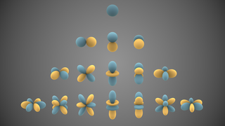
In mathematics and physical science, spherical harmonics are special functions defined on the surface of a sphere. They are often employed in solving partial differential equations in many scientific fields.

In mathematics, the Gibbs phenomenon, discovered by Henry Wilbraham (1848) and rediscovered by J. Willard Gibbs (1899), is the oscillatory behavior of the Fourier series of a piecewise continuously differentiable periodic function around a jump discontinuity. The function's th partial Fourier series produces large peaks around the jump which overshoot and undershoot the function's actual values. This approximation error approaches a limit of about 9% of the jump as more sinusoids are used, though the infinite Fourier series sum does eventually converge almost everywhere except the point of discontinuity.

Inverse trigonometric functions Arcsin, arccos, arctan, etc

In mathematics, the inverse trigonometric functions are the inverse functions of the trigonometric functions. Specifically, they are the inverses of the sine, cosine, tangent, cotangent, secant, and cosecant functions, and are used to obtain an angle from any of the angle's trigonometric ratios. Inverse trigonometric functions are widely used in engineering, navigation, physics, and geometry.

In the mathematical subfields of numerical analysis and mathematical analysis, a trigonometric polynomial is a finite linear combination of functions sin(nx) and cos(nx) with n taking on the values of one or more natural numbers. The coefficients may be taken as real numbers, for real-valued functions. For complex coefficients, there is no difference between such a function and a finite Fourier series.

Sinc function Special mathematical function defined as sin(x)/x

In mathematics, physics and engineering, the sinc function, denoted by sinc(x), has two forms, normalized and unnormalized.

In mathematics, the associated Legendre polynomials are the canonical solutions of the general Legendre equation

Hann function

The Hann function is named after the Austrian meteorologist Julius von Hann. It is a window function used to perform Hann smoothing. The function, with length and amplitude is given by:

In mathematics, a set of n functions f1, f2, ..., fn is unisolvent on a domain Ω if the vectors

Dirichlet kernel

In mathematical analysis, the Dirichlet kernel, named after the German mathematician Peter Gustav Lejeune Dirichlet, is the collection of functions defined as

Exponential response formula

In mathematics, the exponential response formula (ERF), also known as exponential response and complex replacement, is a method used to find a particular solution of a non-homogeneous linear ordinary differential equation of any order. The exponential response formula is applicable to non-homogeneous linear ordinary differential equations with constant coefficients if the function is polynomial, sinusoidal, exponential or the combination of the three. The general solution of a non-homogeneous linear ordinary differential equation is a superposition of the general solution of the associated homogeneous ODE and a particular solution to the non-homogeneous ODE. Alternative methods for solving ordinary differential equations of higher order are method of undetermined coefficients and method of variation of parameters.

References